Introduction
Perceptrons
An artificial neuron is a mathematical function that works as a model of biological neuron which receives one or more inputs and sums them to produce an output. Usually each input is separately weighted, and the sum is passed through a non-linear function known as activation function. A perceptron is a type of artificial neuron. Perceptron takes several binary inputs \(x_1, x_2, \ldots\) and produces a single binary output.

In order to compute the output, Rosenblatt proposed a simple rule to compute the output by using weights \(w_1,w_2,\ldots\), which are real numbers expressing the impotence of the respective input to the output. The neuron's output, 0 or 1, is determined by whether the weighted sum \(\sum_j w_j x_j\) is less than or greater than some threshold value. The threshold is a real number which is a parameter of the neuron.
$$ \text{output} = \begin{cases} 0 & \text{if } \sum_j w_j x_j \leq \text{ threshold} \\ 1 & \text{if } \sum_j w_j x_j \gt \text{ threshold} \tag{1} \end{cases} $$
A perceptron is a device that makes decisions by weighing up evidence. A network of perceptrons can make sophisticated decisions.
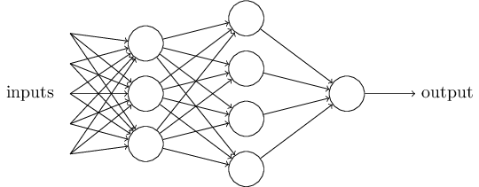
The first layer of perceptrons is making three very simple decisions by weighing the input evidence. The second layer can make a decision at a more complex and more abstract level than perceptrons in the first layer. And even more complex decisions can be made by the perceptron in the third layer. The perceptrons have single output which is distributed as input to other perceptrons.
We can simplify the way we describe perceptrons. We can write the sum as a dot product of two vectors: \(w \cdot x \equiv \sum_j w_j x_j\). Also, we can move the threshold to the other side of the equation, and replace it with perceptron's bias, \(b \equiv -\text{threshold}\).
$$ \text{output} = \begin{cases} 0 & \text{if } w \cdot x + b \leq 0 \\ 1 & \text{if } w \cdot x + b \gt 0 \tag{2} \end{cases} $$
Bias is a measure of how easy it is to get the perceptron to output a 1, or, in biological terms, to fire. Using bias instead of threshold makes notation easier. If the bias is large and positive, it is easy for the perceptron to output 1, whereas if it is large and negative, the output 1 is difficult.
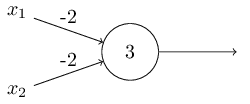
Another way perceptrons can be used is to compute the elementary logical functions we usually think of as the basis of computation, such as And, Or, and Nand gates. For example, suppose we have a perceptron with two inputs, each with weight \(-2\), and an overall bias of \(3\). This perceptron implements a Nand gate:
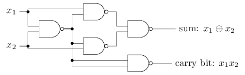
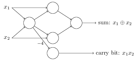
It is possible to build an entire computer with only Nand gates, therefore a perceptron network is universal for computation. For example, we can use Nand gates to build a circuit which adds two bits, \(x_1\) and \(x_2\).
To get an equivalent network of perceptrons, we replace all the Nand gates by perceptrons with two inputs, each with weight \(-2\), and an overall bias of \(3\).
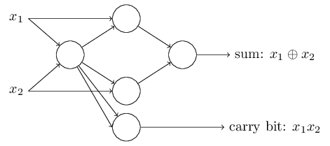
Alternatively, we can modify the network by merging two outputs from the leftmost perceptron that are used as inputs to the bottommost perceptron into a single connection with a weight of \(-4\) instead of two connections with \(-2\) weights.
Unlike conventional logic gates, artificial neurons can learn to solve problems without direct intervention by a programmer by adjusting its weights and biases.
Sigmoid neurons
One way to make learning work is to make a small change in some weight or bias in the network that will cause a small corresponding change in the output from the network.
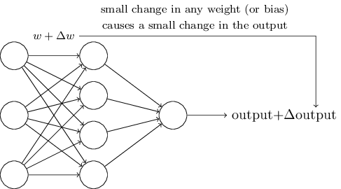
However, it is difficult to do this with perceptrons, because a small change in weight or bias may cause the perceptron's output to flip from, say, 0 to 1. That flip may change the behavior of the rest of the network in some complicated way. We overcome this problem by introducing a new type of artificial neuron called a sigmoid neuron (also called logistic neuron). Sigmoid neurons are similar to perceptrons, but modified so that small changes in their weights and biases cause only a small change in their output. We depict sigmoid neurons the same way as perceptrons:
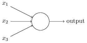
Just like a perceptron, the sigmoid neuron has inputs, \(x_1, x_2, \ldots\). But instead of being just 0 or 1, these inputs can also take on any values between 0 and 1. Also, just like a perceptron, the sigmoid neuron has weights \(w_1, w_2, \ldots\) for each input and an overall bias \(b\). But the output is not 0 or 1. Instead it is \(\sigma(w \cdot x+b)\), where \(\sigma\) is called the sigmoid function, and it is defined by:
$$ \begin{align} \sigma(z) \equiv \frac{1}{1+e^{-z}}. \tag{3} \end{align} $$
This sigmoid function is also called an activation function because it determines the output of a sigmoid neuron. The sigmoid function \(\sigma\) takes the weighted input \(z\), which we define as:
$$ \begin{align} z \equiv \sum_j w_j x_j + b. \tag{4} \end{align} $$
Perceptrons and sigmoid neurons have much in common: they behave in a similar way for large positive and negative values. The difference is seen only when \(w_1,w_2,\ldots\) is of modest size.
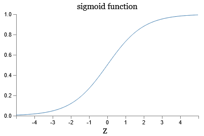
The shape of a sigmoid function is a smoothed out version of a step function:
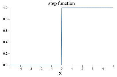
If \(\sigma\) had been a step function, then the sigmoid neuron would be a perceptron, since the output would be 1 or 0 depending on whether \(w\cdot x+b\) was positive or negative (with slight modifications to the step function at 0). The smoothness of \(\sigma\) means that small changes \(\Delta w_j\) in the weights and \(\Delta b\) in the bias will produce a small change \(\Delta \text{output}\) in the output from the neuron, which we can find by a linear approximation as
$$ \begin{align} \Delta \text{output} \approx \left( \sum_j \frac{\partial \, \text{output}}{\partial \, w_j} \Delta w_j \right) + \frac{\partial \, \text{output}}{\partial \, b} \Delta b, \tag{5} \end{align} $$
where the sum is over all the weights, \(w_j\), and \(\partial \,\text{output} / \partial \, w_j\) and \(\partial \, \text{output} /\partial \, b\) denote partial derivatives of the output with respect to \(w_j\) and \(b\), respectively.
It's the shape of \(\sigma\) that matters, and not its exact form. We will later consider neurons where the output is \(f(w \cdot x + b)\) for some other activation function \(f\). Using \(\sigma\) will simplify the algebra because exponentials are easy to differentiate.
The architecture of neural networks
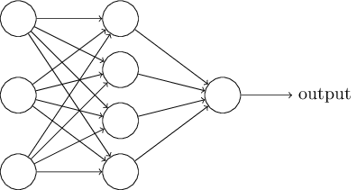
The leftmost layer in the network is called the input layer, and the neurons within the layer are called input neurons. The rightmost or output layer contains the output neurons, or a single neuron as in this case. The middle layer is called a hidden layer, because the neurons in this layer do not directly interact with the outside environment.
Some networks have multiple hidden layers. For example, the following four-layer network has two hidden layers:
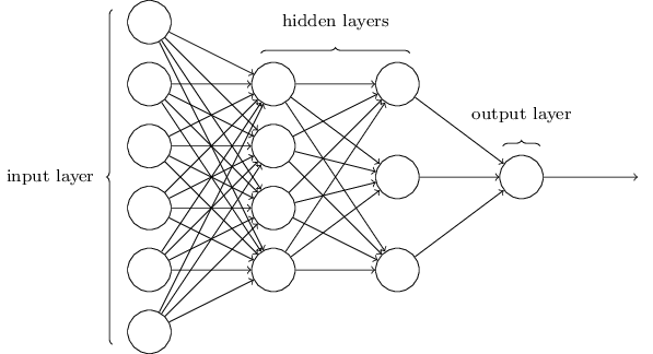
Such multiple layer networks are sometimes called multilayer perceptrons or MLPs, despite being made up of sigmoid neurons, not perceptrons.
The design of input and output layers is often straightforward. For example, we encode 64 by 64 pixel image into 4096 neurons with intensities scaled appropriately between 0 and 1. The output layer may contain just a single neuron, with output values of less than 0.5 indicating "input image is not a 9", and values greater than 0.5 indicating "input image is a 9". In contrast, the design of the hidden layers is based on heuristics.
Up to now we've been discussing feedforward neural networks, where the output from one layer is used as input to the next layer. There are no loops in the network. However, there are other models of artificial networks in which feedback loops are possible. These models are called recurrent neural networks. The idea in these models is to have neurons which fire for some limited duration of time, before becoming quiescent. That firing can stimulate other neurons, which may fire a little later, also for a limited duration. That causes still more neurons to fire, and so over time we get a cascade of neurons firing. Loops don't cause problems in such a model, since a neuron's output only affects its input at some later time, not instantaneously.
A simple neural network example
We will illustrate how neural networks operate by giving an example of a simple network to classify handwritten digits. To recognize individual digits we will use a three-layer neural network:
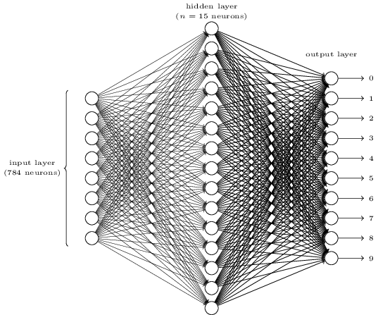
The input layer of the network contains neurons encoding the values of the input pixels. Our training data for the network consist of many 28 by 28 pixel images of scanned handwritten digits, and so the input layer contains \(784 = 28 \times 28\) neurons. The input pixels are grayscale, with a value of 0.0 representing white, a value of 1.0 representing black, and in between values representing gradually darkening shades of gray.
The second layer of the network is a hidden layer. We denote the number of neurons in this hidden layer by \(n\), and we'll experiment with different values for \(n\). In this example \(n = 15\) neurons.
The output layer of the network contains 10 neurons. We number the output neurons from 0 through 9, and figure out which neuron has the highest activation value. If the first neuron fires, i.e. has an input \(\approx 1\), then that will indicate that the network thinks the digit is a 0.
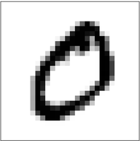
The first output neuron is trying to decide whether or not the digit is 0. It does this by weighing up evidence from the hidden layer of neurons. Those hidden neurons are detecting patterns in the image by heavily weighing up input pixels which overlap with a specific pattern, and only lightly weighing the other inputs. For example, the first hidden neuron may detect the presence of the following pattern:

In a similar way, the second, third, and fourth neurons in the hidden layer may detect whether or not the following images are present:
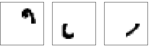
These four images together make up the image of the digit 0. So if all four of these hidden neurons are firing, then we can conclude that the digit is a 0. However, we can use many other ways to come to the same conclusion (through translations or slight distortions).
Adapted from Michael A. Nielsen, "Neural Networks and Deep Learning"