Implementation
Network class
We will be using MNIST data which consists of 60,000 training images and 10,000 test images. We will further separate 60,000 training set into two parts: a set of 50,000 images which we will use to train our network, and a separate 10,000 images validation set. We will use validation set later to figure out how to set certain hyper-parameters of the neural network, such as the learning rate which are not directly selected by our learning algorithm. We will also need Numpy library in Python which will allow us to do fast linear algebra operations.
The center of the neural network code is the Network class, which we use to represent a neural network.
import numpy as np

class Network(object):
    def __init__(self, sizes, seed=None):
        """The list ``sizes`` contains the number of neurons in the
        respective layers of the network. For example, if the list
        was [3, 4, 2] then it would be a three-layer network, with the
        first layer containing 3 neurons, the second layer 4 neurons,
        and the third layer 2 neurons. The biases and weights for the
        network are initialized randomly, using a Gaussian
        distribution with mean 0 and variance 1. Note that the first
        layer is assumed to be an input layer, and by convention we
        won't set any biases for those neurons, since biases are only
        ever used in computing the outputs from later layers. Integer
        ``seed`` may be provided to achieve reproducible results."""
        self.rng = np.random.default_rng(seed)
        self.num_layers = len(sizes)
        self.biases = [self.rng.standard_normal(size=(j, 1), dtype=np.float64)
            for j in sizes[1:]]
        self.weights = [self.rng.standard_normal(size=(j, k), dtype=np.float64)
            for j, k in zip(sizes[1:], sizes[:-1])]
In the code, sizes is a list that contains the number of neurons in respective layers. For example, if we want to create a Network() object with 3 neurons in the first layer, 4 neurons in the second layer, and 2 neurons in the third layer, we will initialize the class object as following:
net = Network([3, 4, 2])
The biases and weights are initialized randomly by using the Numpy rng.standard_normal() function. Later we will find better ways to initialize biases and weights. We assume that the first layer in the network is the input layer, and we omit setting any biases or weights for those neurons, since biases and weights are only ever used in computing the outputs from later layers.
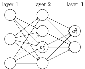
We store biases and weights in Numpy arrays. For example, net.weights[1] may store the following weights connecting the second and the third layers of neurons ($w^3$):
     k=1     k=2      k=3     k=4
[[ 0.3490, 0.2552,  1.7718, -0.6382 ],  j=1
 [ 1.5340, 0.2998, -1.0761, -1.4656 ]]  j=2
net.weights[1] is a matrix such that $w_{jk}$ is the weight for the connection between the $k^{\text{th}}$ neuron in the second layer and the $j^{\text{th}}$ neuron in the third layer. The advantage of this ordering is that we can multiply two matrices, weights $w^l$ and activations $a^{l-1}$ directly (recall Equation (7)):
$$ \begin{align} a^{l} = \sigma(w^l a^{l-1}+b^l). \end{align} $$
To illustrate how this works, consider an example of a vector of activations in the second layer ($a^2$):
     k=1
[[0.2871],  j=1
 [0.7834],  j=2
 [0.6244],  j=3
 [0.6702]]  j=4
A vector of biases in the third layer ($b^3$) may look like this:
    k=1
[[-1.3518],  j=1
 [-2.1354]]  j=2
From these vectors and matrices it is easy to see how we can compute a vector of activations for the third layer by using simple matrix multiplication from Equation (7). Note that the sigmoid function $\sigma$ is applied elementwise to the resulting weighted output vector $z^l = w^l a^{l-1}+b^l$. The vector of activations for the third layer ($a^3$) will be the following:
    k=1
[[0.4078],  j=1
 [0.0425]]  j=2
After calculating the weighted input $z$, it is easy to write the code computing the output from a Network() instance. We begin by defining the sigmoid function:
@staticmethod
def sigmoid(z):
    """Returns the sigmoid function."""
    return 1.0/(1.0+np.exp(-z)) # Equation (3)
Note that when the input z is a vector or Numpy array, Numpy automatically applies the function sigmoid() elementwise in vectorized form.
After that we define feedforward() method for the Network() class, which returns an output vector from a given input for each layer:
def feedforward(self, x):
    """Returns a list of ``activations`` in each layer in the network
    for one example."""
    activation = x
    # list to store all the activations, layer by layer
    activations = [x]
    for b, w in zip(self.biases, self.weights):
        z = np.matmul(w, activation) + b # Equation (8)
        activation = self.sigmoid(z) # Equation (7)
        activations.append(activation)
    return activations
Stochastic gradient descent
The main thing that we want our Network() to do is to learn. We will give it an SGD() method which implements stochastic gradient descent:
def SGD(self, train_data, epochs, mini_batch_size, eta,
        test_data=None):
    """Trains the neural network using mini-batch stochastic
    gradient descent. The ``train_data`` is a list of tuples
    ``(x, y)`` representing the training inputs and the
    corresponding desired outputs."""
    n = len(train_data)
    for j in range(epochs):
        # divide train data into mini-batches randomly
        self.rng.shuffle(train_data)
        mini_batches = [train_data[m:m+mini_batch_size]
            for m in range(0, n, mini_batch_size)]
        for mini_batch in mini_batches:
            self.update_mini_batch(mini_batch, mini_batch_size, eta)
        # evaluate metrics
        if test_data:
            correct = self.evaluate(test_data)
            print(f"Epoch {j} : {correct} / {len(test_data)}")
        else:
            print(f"Epoch {j} complete")
The train_data is a list of tuples (x, y), representing the training inputs and corresponding desired outputs. The variables epochs and mini_batch_size are self-explanatory. eta is the learning rate $\eta$. If the optional argument test_data is supplied, then the program will evaluate the network after each epoch of training, and print out partial progress.
The code works as follows. We start each epoch by randomly shuffling the training data, and then we partition data into mini-batches of the appropriate size. After that for each mini-batch we apply a single step of gradient descent. This is done by update_mini_batch(), which updates the network weights and biases according to a single iteration of gradient descent, using just the training data in the mini_batch. Here is the code for the update_mini_batch() method:
def update_mini_batch(self, mini_batch, mini_batch_size, eta):
    """Updates the network's weights and biases by applying
    gradient descent using backpropagation to a single mini-batch.
    The ``mini_batch`` is a list of tuples ``(x, y)``, and ``eta``
    is the learning rate."""
    nabla_b = [np.zeros(b.shape) for b in self.biases]
    nabla_w = [np.zeros(w.shape) for w in self.weights]
    for x, y in mini_batch:
        delta_nabla_b, delta_nabla_w = self.backprop(x, y)
        nabla_b = [nb + dnb for nb, dnb in zip(nabla_b, delta_nabla_b)]
        nabla_w = [nw + dnw for nw, dnw in zip(nabla_w, delta_nabla_w)]
    self.biases = [b-(eta/mini_batch_size)*nb
                    for b, nb in zip(self.biases, nabla_b)] # Equation (25)
    self.weights = [w-(eta/mini_batch_size)*nw
                    for w, nw in zip(self.weights, nabla_w)] # Equation (24)
Most of the work is done by the backpropagation algorithm to figure out partial derivatives $\frac{\partial C_x}{\partial b^l}$ and $\frac{\partial C_x}{\partial w^l}$. So update_mini_batch() works simply by obtaining these gradients from backprop() method for every training example in the mini_batch, summing them up, and then updating self.weights and self.biases appropriately.
Backpropagation
Backpropagation code starts with initializing zero matrices with the shape of the bias and weight matrices. Then we do the feedforward computation to calculate the weighted sums and activations for each layer. After that we compute partial derivatives for the output layer. And finally we go backward and compute the partial derivatives for all the previous layers in the network and return the results.
def backprop(self, x, y):
    """Returns a tuple ``(nabla_b, nabla_w)`` representing the
    gradient for the cost function C_x for one example. ``nabla_b``
    and ``nabla_w`` are layer-by-layer lists of numpy arrays,
    similar to ``self.biases`` and ``self.weights``."""
    nabla_b = [np.zeros(b.shape) for b in self.biases]
    nabla_w = [np.zeros(w.shape) for w in self.weights]
    activations = self.feedforward(x)
    # compute dC/dz, dC/db, and dC/dw for the output layer
    dCda = self.cost_derivative(activations[-1], y) # 1st term of BP1
    sp = self.sigmoid_prime(activations[-1]) # 2nd term of BP1
    delta = np.multiply(dCda, sp) # BP1
    nabla_b[-1] = delta # BP3
    nabla_w[-1] = np.matmul(delta, activations[-2].transpose()) # BP4
    # compute dC/dz, dC/db, and dC/dw for all the previous layers
    for l in range(2, self.num_layers):
        d = np.matmul(self.weights[-l+1].transpose(), delta) # 1st term of BP2
        sp = self.sigmoid_prime(activations[-l]) # 2nd term of BP2
        delta =  np.multiply(d, sp) # BP2
        nabla_b[-l] = delta # BP3
        nabla_w[-l] = np.matmul(delta, activations[-l-1].transpose()) # BP4
    return (nabla_b, nabla_w)
We will also need two derivatives: cost and sigmoid functions for backpropagation and feedforward procedures.
@staticmethod
def cost_derivative(output_activations, y):
    """Returns the vector of partial derivatives dC_x/da
    for the output activations."""
    return (output_activations - y) # Equation (39)
def sigmoid_prime(self, activation):
    """Returns the derivative of the sigmoid function."""
    return activation*(1-activation) # Equation (40)
The evaluate procedure returns the number of correctly identified examples for the testing dataset.
def evaluate(self, test_data):
    """Returns the number of correctly identified examples."""
    test_results = []
    for x, y in test_data:
        activations = self.feedforward(x)
        test_results.append((np.argmax(activations[-1]), y))
    correct = sum(int(x == y) for (x, y) in test_results)
    return correct
Loading MNIST data
We are going to use a helper program to load the MNIST data:
import gzip
import numpy as np

def load_images(file_name):
    """Returns a Numpy array of the images for MNIST data set."""
    with gzip.open(file_name, 'r') as f:
        # first 4 bytes is a magic number
        # MSB is at the beginning of the byte array
        magic_number = int.from_bytes(f.read(4), byteorder='big', signed=False)
        # second 4 bytes is the number of images
        image_count = int.from_bytes(f.read(4), byteorder='big', signed=False)
        # third 4 bytes is the row count
        row_count = int.from_bytes(f.read(4), byteorder='big', signed=False)
        # fourth 4 bytes is the column count
        column_count = int.from_bytes(f.read(4), byteorder='big', signed=False)
        # rest is the image pixel data, each pixel is stored as an unsigned byte
        # pixel values are 0 to 255
        image_data = f.read()
        images = np.frombuffer(image_data, dtype=np.uint8)\
            .reshape((image_count, row_count, column_count))
        return images

def load_labels(file_name):
    """Returns a Numpy array of the labels for MNIST data set."""
    with gzip.open(file_name, 'r') as f:
        # first 4 bytes is a magic number
        # MSB is at the beginning of the byte array
        magic_number = int.from_bytes(f.read(4), byteorder='big', signed=False)
        # second 4 bytes is the number of labels
        label_count = int.from_bytes(f.read(4), byteorder='big', signed=False)
        # rest is the label data, each label is stored as unsigned byte
        # label values are 0 to 9
        label_data = f.read()
        labels = np.frombuffer(label_data, dtype=np.uint8)
        return labels

def load_train_data():
    """Returns the training dataset with specified filenames."""
    train_images = load_images('data/train-images-idx3-ubyte.gz')
    train_labels = load_labels('data/train-labels-idx1-ubyte.gz')
    return (train_images, train_labels)

def load_test_data():
    """Returns the test dataset with specified filenames."""
    test_images = load_images('data/t10k-images-idx3-ubyte.gz')
    test_labels = load_labels('data/t10k-labels-idx1-ubyte.gz')
    return (test_images, test_labels)

def vectorize(labels):
    """Return a 2-dimensional tensor with the second vector
    consisting of 10-dimensional unit vector with a 1.0 in the jth
    position and zeroes elsewhere. This is used to convert a digit
    (0...9) into a corresponding desired output from the neural
    network."""
    result = np.zeros((len(labels), 10, 1), dtype=np.uint8)
    for i in range(len(labels)):
        j = labels[i]
        result[i, j] = 1
    return result

def load_data():
    """Returns preprocessed MNIST dataset for the neural network. ``train_data``
    is a list of tuples (x_train, y_train) representing the training inputs and
    the corresponding labels. len(train_data)=60000. ``test_data`` is a list of
    tuples (x_test, y_test) representing the testing inputs and the
    corresponding labels. len(test_data)=10000. Testing labels are not
    vectorized. x_train.shape=(784, 1), y_train.shape=(10, 1),
    x_test.shape=(784, 1), y_test is an integer."""

    (train_images, train_labels) = load_train_data()
    (test_images, test_labels) = load_test_data()
    # preprocess train data
    train_images = train_images.reshape((60000, 28*28, 1))
    train_images = train_images.astype('float64') / 255
    train_labels = vectorize(train_labels)
    train_data = zip(train_images, train_labels)
    train_data = list(train_data)
    # preprocess test data (labels are not vectorized)
    test_images = test_images.reshape((10000, 28*28, 1))
    test_images = test_images.astype('float64') / 255
    test_data = zip(test_images, test_labels)
    test_data = list(test_data)
    return (train_data, test_data)
The code is available at my GitHub repository.
Running the code
First we will load the MNIST dataset by executing the following command:
import mnist
(train_data, valid_data, test_data) = mnist.load_data()
After loading the MNIST data, we will set up a Network() with a single hidden layer consisting of 15 hidden neurons. For the testing purposes, we can pass a seed value to make sure that the random numbers are initialized from the same pool for different Network() models:
import network
net = Network([784, 15, 10], seed=0)
Finally, we will use stochastic gradient descent to learn from MNIST train_data over 30 epochs, with a mini-batch size of 10, and a learning rate of $\eta = 3.0$:
net.SGD(train_data, 30, 10, 3.0, test_data)
The transcript of learning progress shows us that we started with 9,007 correctly recognized images out of 10,000 at the first epoch, reaching to 9,348 out of 10,000 at the end of the last epoch.
Epoch 0 : 8881 / 10000
Epoch 1 : 9080 / 10000
Epoch 2 : 9144 / 10000
...
Epoch 27 : 9369 / 10000
Epoch 28 : 9334 / 10000
Epoch 29 : 9361 / 10000
We can change the number of hidden neurons to 100 and see what happens.
net = Network([784, 100, 10], seed=0)
net.SGD(train_data, 30, 10, 3.0, test_data)
Unfortunately, the performance has dropped to 87.26 percent:
Epoch 0 : 7488 / 10000
Epoch 1 : 7613 / 10000
Epoch 2 : 7655 / 10000
...
Epoch 27 : 8747 / 10000
Epoch 28 : 8751 / 10000
Epoch 29 : 8747 / 10000
Adjusting hyper-parameters
To obtain these accuracies we made specific choices for the number of epochs of training, the mini-batch size, and the learning rate $\eta$. These are called hyper-parameters for our neural network, which are distinct from the parameters (weights and biases) learned by our learning algorithm. If we choose our hyper-parameters poorly, we can get bad results. For example, if we choose the learning rate to be $\eta = 0.001$,
net = Network([784, 15, 10], seed=0)
net.SGD(train_data, 30, 10, 0.001, test_data)
the results will be much less encouraging:
Epoch 0 : 816 / 10000
Epoch 1 : 1040 / 10000
Epoch 2 : 1217 / 10000
...
Epoch 27 : 2438 / 10000
Epoch 28 : 2487 / 10000
Epoch 29 : 2532 / 10000
In general, debugging a neural network can be challenging when initial choice of hyper-parameters produces results no better than random noise. Suppose we try to set the learning rate to $\eta = 100$:
net = Network([784, 15, 10], seed=0)
net.SGD(train_data, 30, 10, 100, test_data)
The results show that we have gone too far, and our learning rate is too high:
Epoch 0 : 958 / 10000
Epoch 1 : 958 / 10000
Epoch 2 : 890 / 10000
...
Epoch 27 : 890 / 10000
Epoch 28 : 890 / 10000
Epoch 29 : 890 / 10000
Now if we were coming to this problem for the first time, the output would not tell us much about how we can improve the results. We might worry not only about the learning rate, but about every other aspect of our neural network:
- Did we initialized the weights and biases in the way that makes it hard for the network to learn?
- Maybe we don't have enough training data to get meaningful learning?
- Perhaps we haven't run for enough epochs?
- Maybe it's impossible for a neural network with this architecture to learn to recognize handwritten digits?
- Learning rate is too high?
- Learning rate is too low?
Adapted from Michael A. Nielsen, "Neural Networks and Deep Learning"