Principal component analysis

Feature extraction methods transform a dataset into a new feature subspace of lower dimensionality by keeping the most relevant information. It helps store and analyze data with better efficiency.

Principal component analysis (PCA) is an unsupervised linear transformation method that is used for feature extraction and dimensionality reduction. Other applications of PCA include exploratory data analysis, denoising of signals in stock market trading, and the analysis of genome data.

PCA finds the directions of maximum variance in high-dimensional data and projects the data onto a new subspace with equal or fewer dimensions. PCA takes a feature vector $x \in \mathbb{R}^d$, transforms it by a transformation matrix $W \in \mathbb{R}^{d \times k}$, which results in the output vector $z \in \mathbb{R}^k$.

$$xW = z$$

Understanding variance

The first principal component has the largest variance given the constraint that all principal components are orthogonal to each other. Thus, the first principal component is the most valuable for clustering the data.

Variance is the expectation of the squared deviation of a random variable from its population or sample mean.

$$\sigma^2 = \frac{1}{n-1} \sum_{i=1}^n (x_i - \bar x)^2$$

It is a measure of how far a set of numbers is spread out from their average value.

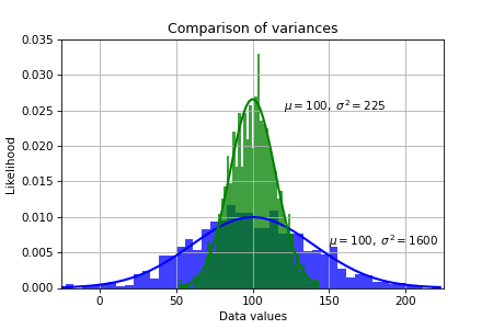
Variance is the square of standard deviation, and it is also a covariance of a random variable with itself. We ordinarily measure the sample variance as an approximation to the population variance.

PCA algorithm

1. Standardize the dataset.
2. Construct the covariance matrix.
3. Decompose the covariance matrix into its eigenvalues and eigenvectors.
4. Sort the eigenvalues by decreasing order to rank the corresponding eigenvectors.
5. Select $k$ largest eigenvalues and eigenvectors, where $k$ corresponds to the dimensionality of the new feature space.
6. Construct a projection matrix $W$ from $k$ eigenvectors.
7. Transform the $d$-dimensional input dataset $X$ to obtain the new $k$-dimensional feature subspace.

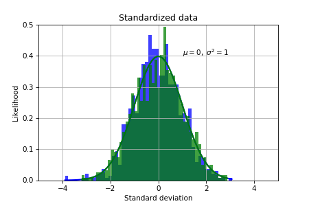
Standardizing the dataset

PCA directions are highly sensitive to data scaling, therefore we need to standardize the input features before using PCA. First we import the Wine dataset as an example:

import pandas as pd

df_wine = pd.read_csv('https://archive.ics.uci.edu/ml/'
                      'machine-learning-databases/wine/wine.data',
                      header=None)
X, y = df_wine.iloc[:, 1:].values, df_wine.iloc[:, 0].values

Then we split the dataset into 70% training and 30% test subsets:

import numpy as np

n = len(y)
seed = 0
rng = np.random.default_rng(seed)
mask = rng.permutation(list(range(n)))

test_ratio = 0.3
n_test = int(n*test_ratio)
n_train = n-n_test

X_train, y_train = X[mask][:n_train], y[mask][:n_train]
X_test, y_test = X[mask][n_train:], y[mask][n_train:]

Finally, we standardize the data to measure how many standard deviations the values are from the zero mean:

mu = np.mean(X_train, axis=0)
sigma = np.std(X_train, axis=0)

X_train_std = (X_train-mu)/sigma
X_test_std = (X_test-mu)/sigma

Constructing the covariance matrix

Next we will construct the covariance matrix, which stores covariances between different features. Covariance between two features $x_j$ and $x_k$ in samples is calculated by the following formula:

$$\sigma_{jk} = \frac{1}{n-1} \sum_{i=1}^n (x_j^{(i)}-\mu_j)(x_k^{(i)}-\mu_k)$$

where $n$ is the number of data points, $\mu_j$ is the mean of data along feature $x_j$, and $\mu_k$ is the mean of data along feature $x_k$. We can also calculate the covariance matrix in vectorized form (with broadcasting) as the following:

$$\Sigma = \begin{bmatrix} \sigma_{1}^2 & \sigma_{12} & \cdots & \sigma_{1d}\\ \sigma_{21} & \sigma_{2}^2 & \cdots & \sigma_{2d}\\ \vdots & \vdots & \vdots & \vdots\\ \sigma_{d1} & \sigma_{d2} & \cdots & \sigma_{d}^2\\ \end{bmatrix} = \frac{1}{n-1} (X_{\text{train}}-m_X)^T (X_{\text{train}}-m_X)$$

where $m_X$ is the horizontal vector of mean values calculated along each feature. Note that if the two features are uncorrelated, their covariance is zero.

cov_mat = (X_train_std.T @ X_train_std)/(X_train_std.shape[0]-1)

Covariance matrix $\Sigma$ is a square $d \times d$ symmetric matrix. Therefore, it has the following properties:

1. All the eigenvalues of $\Sigma$ are real numbers.
2. The dimension of an eigenspace of $\Sigma$ is the multiplicity of the eigenvalue as a root of the characteristic equation.
3. The eigenspaces of $\Sigma$ are orthogonal.
4. $\Sigma$ has $d$ linearly independent eigenvectors.

Eigenvalues and eigenvectors

Let $A$ be an $n \times n$ matrix. A scalar $\lambda$ is called an eigenvalue of $A$ if there exists a nonzero vector $x$ in $\mathbb{R}^n$ such that

$$Ax = \lambda x$$

$$Ax -\lambda x = 0$$

$$(A -\lambda I_n) x = 0$$

Nonzero solutions exist only if the matrix of coefficients is singular. The determinant $|A -\lambda I_n|$ is called the characteristic polynomial, and the equation $|A -\lambda I_n| = 0$ is called the characteristic equation. From the characteristic equation we first find the eigenvalues, and then solve the system of linear equations to find the corresponding eigenvectors.

Eigendecomposition of the covariance matrix

Now we need to find the set of eigenvalues and eigenvectors:

$$\Sigma v = \lambda v$$

We will perform eigendecomposition using linalg.eig function from Numpy library:

eigen_vals, eigen_vecs = np.linalg.eig(cov_mat)

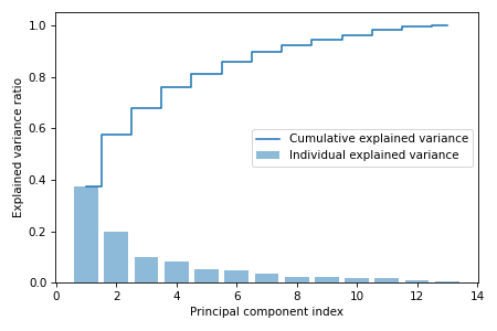
Total and explained variance

Our goal is to reduce the dimensionality of the dataset, and we do it by selecting a subset of eigenvectors which are called principal components that contains most of the variance. The eigenvalues define the magnitude of the eigenvectors, therefore we need to sort them by decreasing order. From the geometric perspective, eigenvalues are the sums of square distances from the origin to the projection of each data point on the best-fit line in one dimension. Eigenvalues determine the proportion of variation that each principal component accounts for.

But first we need to find explained variance ratio, which is the fraction of an eigenvalue to the total sum of the eigenvalues:

$$\text{Explained variance ratio} = \frac{\lambda_i}{\sum_{j=1}^d \lambda_j}$$

eigen_vals_tot = eigen_vals.sum()
var_exp = [(i / eigen_vals_tot) for i in sorted(eigen_vals, reverse=True)]
cum_var_exp = np.cumsum(var_exp)

We can now plot the cumulative sum of explained variances which is called the Scree plot to understand the contribution of principal components to variance in the data.

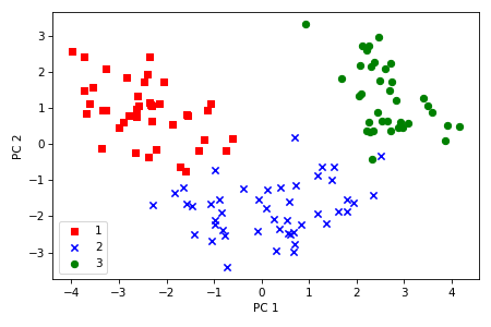
Feature transformation

Our next task is to sort the eigenvectors by decreasing order of the eigenvalues and choose the two eigenvectors (principal components) that have the largest eigenvalues, which captures about 60 percent of the variance in the dataset. We choose two principal components for the purpose of illustration, however in practice the number of principal components $k$ has to be determined by a trade-off between computational efficiency and performance of the classifier. The number of principal components is limited by the number of features or the number of samples, whichever is smaller.

Each eigenvector component is called the loading score for each feature. The eigenvector is thus the linear combination of the features.

eigen_pairs = [(np.abs(eigen_vals[i]), eigen_vecs[:, i])
               for i in range(len(eigen_vals))]

eigen_pairs.sort(key=lambda k: k[0], reverse=True)

W = np.vstack((eigen_pairs[0][1], eigen_pairs[1][1])).T

We have obtained a $13 \times 2$ projection matrix $W$ from the first two eigenvectors. Now we can transform the dataset onto the PCA subspace:

$$X' = XW$$

X_train_pca = X_train_std @ W

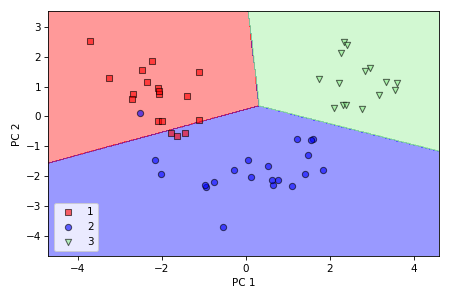
We can also visualize the data spread in a plot along two axes which correspond to two principal components. We can observe that now it is possible to successfully separate the classes with a linear classifier.

PCA in scikit-learn

As before, we first need to import, split, and standardize the dataset

import pandas as pd

df_wine = pd.read_csv('https://archive.ics.uci.edu/ml/'
                      'machine-learning-databases/wine/wine.data',
                      header=None)
X, y = df_wine.iloc[:, 1:].values, df_wine.iloc[:, 0].values

from sklearn.model_selection import train_test_split

X_train, X_test, y_train, y_test = \
train_test_split(X, y, test_size=0.3, stratify=y, random_state=0)

from sklearn.preprocessing import StandardScaler

sc = StandardScaler()
X_train_std = sc.fit_transform(X_train)
X_test_std = sc.transform(X_test)

The PCA transformation with two principal components is done the following way:

from sklearn.decomposition import PCA

pca = PCA(n_components=2)
X_train_pca = pca.fit_transform(X_train_std)
X_test_pca = pca.transform(X_test_std)
var_exp = pca.explained_variance_ratio_

Finally, we will try to fit a simple logistic regression model on the reduced dataset and evaluate the model on the training set.

from sklearn.linear_model import LogisticRegression

lr = LogisticRegression(multi_class='ovr', random_state=1, solver='lbfgs')
lr = lr.fit(X_train_pca, y_train)
test_score = np.sum(lr.predict(X_test_pca) == y_test)/y_test.shape[0]

We obtained about 93% accuracy on unseen data, having only 4 misclassified test examples.

The supporting code for this article is available on Github.

Adapted from Sebastian Raschka & Vahid Mirjalili, "Python Machine Learning".