Choosing hyper-parameters

Strategy

Suppose we have just started attacking the problem and don't know which hyper-parameters to set. We will try to train our neural network on MNIST data for 30 epochs using cross-entropy with 30 hidden neurons and a mini-batch size of 10. But this time we will choose a learning rate $\eta=10.0$ and regularization parameter $\lambda=1000.0$.

(training_data, validation_data, test_data) = mnist.load_matrix_data()
net3 = network3.Network([784, 30, 10])
(training_cost,
training_accuracy,
evaluation_cost,
evaluation_accuracy) = net3.SGD(training_data, 30, 10, 10.0,
    lmbda = 1000.0,
    evaluation_data=validation_data,
    monitor_evaluation_accuracy=True)

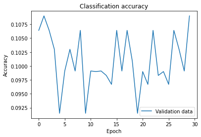
The result is that the classification accuracy is no better than chance: the network acts as a random noise generator.

Our broad strategy of using neural networks to attack a new problem is first to get any learning at all to achieve results better than chance. For this purpose we simplify the problem, for example, by stripping the training data to only zeros and ones. Then we try to train the network to distinguish zeros from ones. It is an easier problem with reduced amount of training data that allows much more rapid experimentation.

We can further speed up experimentation by choosing a simpler network. If we believe that [784, 10] network can deliver better-than-chance classification of MNIST digits, then we can begin our experimentation with such a network. It will be much faster than training [784, 30, 10] network, and we can restore the complexity of the network later.

We can also increase the frequency of monitoring. We can get feedback by monitoring the validation accuracy more often, for example, after every 1,000 training images instead of after every 50,000 training images. Moreover, instead of using the full 10,000 image validation set to monitor performance, we can get a much faster estimate using just 100 validation images.

(training_data, validation_data, test_data) = mnist.load_matrix_data()
(X, Y) = training_data
(Xv, Yv) = validation_data
net3 = network3.Network([784, 10])
(training_cost,
training_accuracy,
evaluation_cost,
evaluation_accuracy) = net3.SGD((X[:,:1000],Y[:,:1000]), 30, 10, 10.0,
    lmbda = 1000.0,
    evaluation_data=(Xv[:,:100],Yv[:100]),
    monitor_evaluation_accuracy=True)

Now we are getting the results much faster so we can get the feedback more quickly and have a room to experiment with other choices of hyper-parameters. However, we need to change the regularization parameter to lmbda = 20.0 so that the weight decays at the same rate as before because we have reduce the number of training examples.

Suppose that at this point we decide that our learning rate $\eta$ should be higher so we set it to $\eta=100.0$ and see what happens:

(training_data, validation_data, test_data) = mnist.load_matrix_data()
(X, Y) = training_data
(Xv, Yv) = validation_data
net3 = network3.Network([784, 10])
(training_cost,
training_accuracy,
evaluation_cost,
evaluation_accuracy) = net3.SGD((X[:,:1000],Y[:,:1000]), 30, 10, 100.0,
    lmbda = 1000.0,
    evaluation_data=(Xv[:,:100],Yv[:100]),
    monitor_evaluation_accuracy=True)

We observe that the results are bad, so instead we dial down the learning rate to $\eta=1.0$. This gives some better results. And so we continue adjusting each hyper-parameter one-by-one and look at the results. Once we have found an improvement of $\eta$, we can move on to find a good value for $\lambda$. Then we can experiment with a more complex architecture, say, a network with 10 hidden neurons. Then adjust $\eta$ and $\lambda$ again. Then increase to 20 hidden neurons. After that adjust other hyper-parameters some more. And so on, at each stage evaluating performance on the validation data to obtain better hyper-parameters. This is a long process, so decreasing the frequency of monitoring helps a lot.

Learning rate

Suppose we run the network with three different learning rates, $\eta=0.025$, $\eta=0.25$, and $\eta=2.5$:

etas = [0.025, 0.25, 2.5]
for eta in etas:
    (training_data, validation_data, test_data) = mnist.load_matrix_data()
    net3 = network3.Network([784, 30, 10])
    (training_cost,
    training_accuracy,
    evaluation_cost,
    evaluation_accuracy) = net3.SGD(training_data, 30, 10, eta,
        lmbda = 5.0,
        evaluation_data=validation_data,
        monitor_training_cost=True)

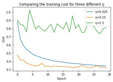
When $\eta=0.025$, the cost decreases smoothly until the final epoch. When $\eta=0.25$, the cost initially decreases, but after about 10 epochs it is near saturation, and most of the changes are merely random oscillations. Finally, with $\eta=2.5$ the cost oscillates from the start. It is likely that the step size is too big for the gradient descent so that it overshoots the minimum.

The procedure to find the best learning rate $\eta$ is the following. First, we estimate the threshold value for $\eta$ at which the cost on the training data immediately begins decreasing, instead of oscillating or increasing. This estimate doesn't need to be accurate. We can estimate the order of magnitude by starting with $\eta=0.01$. If the cost decreases during the first few epochs, then we should successively try $\eta=0.1,1.0,\ldots$ until we find a value for $\eta$ where the cost oscillates or increases during the first few epochs. Alternatively, if the cost oscillates or increases during the first few epochs when $\eta=0.01$, then try $\eta=0.001,0.0001,\ldots$ until we find a value for $\eta$ where the cost decreases during the first few epochs. This procedure will give us an order of magnitude estimate for the threshold value of $\eta$. We may optionally refine the estimate to pick out the largest value of $\eta$ at which the cost decreases during the first few epochs. This gives us an estimate for the threshold value of $\eta$.

The actual value of $\eta$ that we use should be no larger than the threshold value. If the value of $\eta$ is to remain usable over many epochs then we likely want to use a value for $\eta$ that is smaller, say a factor of two below the threshold. This will allow us to train for many epochs without causing too much of a slowdown in learning.

metric = {}
etas = [0.2, 0.3, 0.4, 0.5, 0.6]
for eta in etas:
    (training_data, validation_data, test_data) = mnist.load_matrix_data()
    net3 = network3.Network([784, 30, 10])
    (training_cost,
    training_accuracy,
    evaluation_cost,
    evaluation_accuracy) = net3.SGD(training_data, 30, 10, eta,
        lmbda = 5.0,
        evaluation_data=validation_data,
        monitor_training_cost=True)
    metric['$\eta$='+str(eta)] = training_cost

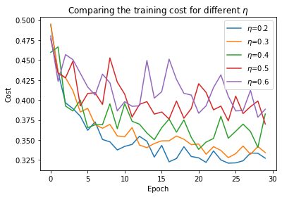
Following this procedure we can find the threshold value of $\eta=0.5$, and this suggests to use the value $\eta=0.25$ as our learning rate.

We are using the training data to choose the learning rate because the primary purpose of the learning rate is to control the step size in gradient descent, and monitoring the training cost is the best way to detect if the step size is too big. We will use accuracy on the validation data to pick other hyper-parameters, such as the regularization hyper-parameter, the mini-batch size, the number of layers and hidden neurons, and so on.

Number of training epochs

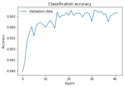
We are going to use the hyper-parameter early stopping to determine the number of training epochs. Early stopping means that we should compute the classification accuracy on the validation data. When that stops improving, we terminate the learning process. Note that the accuracy can oscillate even though the overall trend is to improve. If we stop the first time the accuracy decreases then we almost certainly stop when there is more improvements to be found. A better strategy is to terminate if the best classification accuracy doesn't improve for quite some time. A good starting point is no-improvement-one-in-ten rule. However, networks can also plateau near a particular point for some time, only to continue improving again. We can experiment with other no-improvement-in-n rules.

(training_data, validation_data, test_data) = mnist.load_matrix_data()
net3 = network3.Network([784, 30, 10])
(training_cost,
training_accuracy,
evaluation_cost,
evaluation_accuracy) = net3.SGD(training_data, 100, 10, 0.25,
    lmbda = 5.0,
    evaluation_data=validation_data,
    monitor_evaluation_accuracy=True,
    early_stopping_n = 10)

Learning rate schedule

At the beginning of the learning process the weights are usually badly wrong. For this reason it is reasonable to use a large learning rate that causes the weights to change quickly. We can hold the learning rate constant until the validation accuracy starts to get worse. Then we decrease the learning rate by some amount, say, a factor of two or ten. We repeat this many times until the learning rate is a factor of 1,024 or 1,000 times lower than the initial value. Then we terminate.

# before epochs loop
original_eta = eta

# --- some code ---

# at the end of each epoch
if accuracy >= best_accuracy:
    best_accuracy = accuracy
else:
    eta = eta/2
    print("Update learning rate: {}".format(eta))
if (original_eta/eta > 1024):
    return training_cost, training_accuracy, \
        evaluation_cost, evaluation_accuracy

Regularization parameter

We start initially with no regularization ($\lambda=0.0$), and first determine the value for $\eta$ as described above. Using that choice of $\eta$, we can now use the validation data to select a good value for $\lambda$. Starting with $\lambda=1.0$, we increase or decrease by factors of 10 as needed to improve the performance on the validation data. Once we have found a good order of magnitude, we can fine-tune the value of $\lambda$. After all of that, we should return and re-optimize $\eta$ again.

lmbdas = [1.0, 0.1, 10, 100, 0.01]
training_cost_metric = {}
training_accuracy_metric = {}
evaluation_cost_metric = {}
evaluation_accuracy_metric = {}
for lmbda in lmbdas:
    (training_data, validation_data, test_data) = mnist.load_matrix_data()
    net3 = network3.Network([784, 30, 10])
    (training_cost,
    training_accuracy,
    evaluation_cost,
    evaluation_accuracy) = net3.SGD(training_data, 30, 10, 0.25,
        lmbda = lmbda,
        evaluation_data=validation_data,
        monitor_training_cost=True,
        monitor_training_accuracy=True,
        monitor_evaluation_cost=True,
        monitor_evaluation_accuracy=True)
    cost_metric = {}
    training_cost_metric['$\lambda$='+str(lmbda)] = training_cost
    training_accuracy_metric['$\lambda$='+str(lmbda)] = training_accuracy
    evaluation_cost_metric['$\lambda$='+str(lmbda)] = evaluation_cost
    evaluation_accuracy_metric['$\lambda$='+str(lmbda)] = evaluation_accuracy

Mini-batch size

Suppose that we are doing online learning (mini-batch size of 1). Since the mini-batches contain only a single training example, we worry that it will cause significant errors in the estimate of the gradient. In fact, the errors turn out to not be such a problem.

Choosing the best mini-batch size is a compromise. If we choose it to be too small, we don't take advantage of the linear algebra matrix libraries in the hardware. If we choose it to be too large, we won't be updating weights often enough. So we need to make a compromise value which maximizes the speed of learning. Fortunately, the choice of mini-batch size is relatively independent of the other hyper-parameters.

We can start by using some acceptable values for the other hyper-parameters first, and then try a number of different mini-batch sizes, scaling $\eta$ by the size of the mini-batch as the following:

$$ \begin{align} w \rightarrow w' = w-\eta \sum_x \nabla C_x. \tag{101} \end{align} $$

instead of

$$ \begin{align} w \rightarrow w' = w-\eta \frac{1}{m} \sum_x \nabla C_x \tag{102} \end{align} $$

After that we plot the validation accuracy versus time (real elapsed time, not epochs!), and choose which mini-batch size gives the most rapid improvement in performance.

Automated techniques

The process of manually optimizing hyper-parameters helps to build up a feel for how neural networks behave. However, a great deal of work has been done to automate this process. The most common technique is grid search, which systematically searches through a grid in hyper-parameter space.

Variations on stochastic gradient descent

• Hessian technique

• Momentum-based gradient descent

Adapted from Michael A. Nielsen, "Neural Networks and Deep Learning"