Improving learning

Slow learning problem

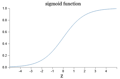
In order to improve the way our neural network learns we first need to understand what is wrong with our previous algorithm. Recall the definition of the sigmoid function from Equation (3) and the shape of it:

$$ \begin{align} \sigma(z) \equiv \frac{1}{1+e^{-z}}. \end{align} $$

Next recall the four fundamental equations of backpropagation:

$$ \begin{align} \delta^L = \frac{\partial C_x}{\partial z^L} &= \nabla_a C_x \odot \sigma'(z^L) \tag{BP1}\\[2ex] \delta^l = \frac{\partial C_x}{\partial z^l} &= ((w^{l+1})^T \delta^{l+1}) \odot \sigma'(z^l) \tag{BP2}\\[2ex] \frac{\partial C_x}{\partial b^l} &= \delta^l \tag{BP3}\\[2ex] \frac{\partial C_x}{\partial w^l} &= \delta^l (a^{l-1})^T. \tag{BP4} \end{align} $$

We can see that both $\frac{\partial C_x}{\partial b^l}$ and $\frac{\partial C_x}{\partial w^l}$ depend on the derivative of the sigmoid function $\sigma$. From the graph we observe that the slope of the sigmoid function is close to zero when the output of a neuron is close to 0 or 1. In other words, when output activations from the network are close to the desired output, or too far from the desired output, the derivative of $\sigma$ function becomes close to zero, which effectively slows down the learning process.

Cross-entropy cost function

In order to mitigate the slow learning problem, we introduce the cross-entropy cost function and define it by the following equation:

$$ \begin{align} C = -\frac{1}{n} \sum_x \sum_j \left[y_j \ln a^L_j + (1-y_j) \ln (1-a^L_j) \right], \tag{64} \end{align} $$

where $n$ is the total number of training examples; the sum is over individual training examples $x$ and individual neurons $j$ in the output layer; $y = y(x)$ is the corresponding desired output; $L$ denotes the number of layers in the network; and $a^L = a^L(x)$ is the vector of activations output from the network when $x$ is input. The output $a$ depends on $x,$ $w,$ and $b$.

We can rewrite the cross-entropy cost function for a single training example $x$ as

$$ \begin{align} C_x = -\sum_j \left[y_j \ln a^L_j + (1-y_j) \ln (1-a^L_j) \right]. \tag{65} \end{align} $$

Notice that the cross-entropy cost function is non-negative and tends toward zero as the neuron's output activations $a$ get closer to the desired output $y$. We expect both of these properties from a cost function, and the quadratic cost function also satisfies them. However, unlike the quadratic cost function, the cross-entropy cost function avoids slowing the learning process because its derivative cancels out the derivative of the sigmoid function in Equation (BP1) (more about this below). We can analyze how the cross-entropy function behaves by substituting various values of $y$ and $a$:

$$ \begin{align} & y = 0, a \approx 0 \Rightarrow C \to 0\\ & y = 1, a \approx 1 \Rightarrow C \to 0\\ & y = 1, a \approx 0 \Rightarrow C \to \infty\\ & y = 0, a \approx 1 \Rightarrow C \to \infty\\ \end{align} $$

If the output neurons are sigmoid neurons, it is always better to use the cross-entropy instead of the quadratic cost. The reason is that when initial random choices for weights and biases are decisively wrong for some training input, so that an output neuron is saturated near 1 when it should be 0 or vice versa, then the quadratic cost will slow down the learning process. This happens because the derivative of the sigmoid function in Equation (BP1) will be close to zero. Now we will show that cross-entropy cost function could be used for any values of $a$ and $y$ in the interval between $0$ and $1$. Recall from Equation (40) that

$$ \begin{align} \sigma'(z_j^L) = a_j^L(1 - a_j^L). \end{align} $$

To show that cross entropy is minimized for any value of $y_j$ between $0$ and $1$ when $a(z_j^L) = \sigma (z_j^L)$, we take the derivative of the cross-entropy cost function with respect to $z$:

$$ \begin{align} \frac{\partial C}{\partial z_j^L} & = -\frac{1}{n} \sum_x \left[y_j \frac{\sigma'(z_j^L)}{\sigma(z_j^L)} - (1 - y_j) \frac{\sigma'(z_j^L)}{1 - \sigma(z_j^L)}\right]\\[2ex] & = -\frac{1}{n} \sum_x \left[y_j \frac{\sigma(z_j^L)(1 - \sigma(z_j^L))}{\sigma(z_j^L)} - (1 - y_j) \frac{\sigma(z_j^L)(1 - \sigma(z_j^L))}{1 - \sigma(z_j^L)}\right]\\[2ex] & = -\frac{1}{n} \sum_x \left[y_j (1 - \sigma(z_j^L)) - (1-y_j) \sigma(z_j^L)\right]\\[2ex] & = -\frac{1}{n} \sum_x \left[y_j - y_j \sigma(z_j^L) - \sigma(z_j^L) + y_j \sigma(z_j^L)\right]\\[2ex] & = -\frac{1}{n} \sum_x \left[y_j - \sigma(z_j^L)\right] \tag{66} \end{align} $$

We know from calculus that the cross-entropy function will have an extreme value when its first derivative equals zero, that is when $\sigma(z_j^L) = y_j$. To show that this extremum is the minimum, we take the second derivative:

$$ \begin{align} \frac{\partial^2 C}{\partial (z_j^L)^2} = \frac{1}{n} \sum_x \left[\sigma(z_j^L) (1 - \sigma(z_j^L))\right] \gt 0 \quad \text{since} \quad 0 \lt \sigma(z_j^L) \lt 1. \tag{67} \end{align} $$

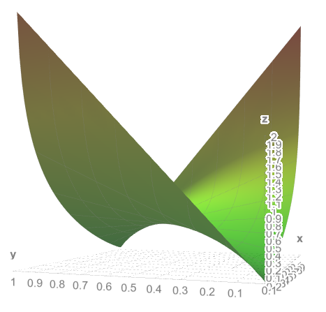
By the second derivative test we conclude that the cross-entropy function is indeed minimized when $\sigma(z_j^L) = y_j$. We can depict the graph of the cross-entropy function as the following:

Recall from Equation (47) that

$$ \begin{align} \frac{\partial z_j^l}{\partial b_j^l} = 1 \end{align} $$

and from Equation (49):

$$ \begin{align} \frac{\partial z_j^l}{\partial w_{jk}^l} = a_k^{l-1}. \end{align} $$

By applying the chain rule, we get the following expressions of the cross-entropy cost function with respect to a particular bias and weight in the output layer of a particular training example:

$$ \begin{align} \frac{\partial C_x}{\partial b_j^L} = a_j^L - y_j. \tag{68} \end{align} $$

$$ \begin{align} \frac{\partial C_x}{\partial w_{jk}^L} = \left( a_j^L - y_j \right) a_k^{L-1}. \tag{69} \end{align} $$

We can also calculate the cross-entropy cost function with respect to biases and weights in the output layer of all training examples as following:

$$ \begin{align} \frac{\partial C}{\partial b_j^L} = \frac1n \sum_x a_j^L - y_j. \tag{70} \end{align} $$

$$ \begin{align} \frac{\partial C}{\partial w_{jk}^L} = \frac1n \sum_x \left( a_j^L - y_j \right) a_k^{L-1}. \tag{71} \end{align} $$

Notice that the term $\sigma'(z_j^L)$ has disappeared, therefore cross-entropy function avoids the problem of slow learning.

Derivation of the cross-entropy cost function

When we realize that the derivative of the sigmoid function slows down learning, we naturally want to use a different cost function that does not have this term. If we consider the quadratic cost function, we have

$$ \begin{align} \frac{\partial C}{\partial b} & = \frac{\partial C}{\partial a} \frac{\partial a}{\partial z}\frac{\partial z}{\partial b}\\[2ex] & = \frac{\partial C}{\partial a} \sigma'(z)\\[2ex] & = \frac{\partial C}{\partial a} a(1-a). \tag{72} \end{align} $$

For the quadratic cost function we have

$$ \begin{align} \frac{\partial C}{\partial a} = a-y, \tag{73} \end{align} $$

and we want to improve it so that the sigmoid prime for $\frac{\partial C}{\partial b}$ disappears:

$$ \begin{align} \frac{\partial C}{\partial a} & = \frac{a-y}{a(1-a)}\\[2ex] \partial C & = \frac{a-y}{a(1-a)}\partial a. \tag{74} \end{align} $$

Integrating this desired expression gives us

$$ \begin{align} \int \partial C & = \int \frac{a-y}{a(1-a)}\partial a\\[2ex] C + c& = \int \frac{a}{a(1-a)}\partial a - \int \frac{y}{a(1-a)}\partial a\\[2ex] C +c & = \int \frac{1}{1-a}\partial a - \int \frac{y}{a}\partial a - \int \frac{y}{1-a}\partial a\\[2ex] C + c & = -\ln |1-a| - y \ln |a| + y \ln |1-a| + d\\[2ex] C + c & = -[y \ln a + (1-y) \ln (1-a)] + d, \tag{75} \end{align} $$

where $c$ and $d$ are the constants of integration. We can remove absolute value sings since $0 \lt a \lt 1$. More information about cross-entropy can be found in Cover and Thomas' Information Theory, chapter 5 about Kraft inequality.

Softmax

The idea behind softmax is to define a different type of the output layer for the neural network. As with a sigmoid layer, we form the weighted inputs $z_j^l = \sum_k w_{jk}^l a_k^{l-1} + b_j^l$ and apply the softmax function to it:

$$ \begin{align} a_j^L = \frac{e^{z_j^L}}{\sum_k e^{z_k^L}}, \tag{76} \end{align} $$

where in the denominator we sum over all the output neurons. The output from the softmax layer is a set of positive numbers which all sum up to 1. It is convenient to think of it as a probability distribution. In contrast, the output from a sigmoid layer will not in general form a probability distribution.

Now we will prove the monotonicity of the softmax:

$$ \begin{align} \frac{\partial a_j^L}{\partial z_k^L} = \frac{ \left(e^{z_j^L}\right)' \sum_k e^{z_k^L} - \left(\sum_k e^{z_k^L}\right)' e^{z_j^L} }{\left(\sum_k e^{z_k^L}\right)^2} \tag{77} \end{align} $$

First consider the case when $j=k$:

$$ \begin{align} \frac{\partial a_j^L}{\partial z_k^L} \bigg|_ {j=k} & = \frac{ \left(e^{z_j^L}\right) \sum_k e^{z_k^L} - e^{2z_j^L} }{\left(\sum_k e^{z_k^L}\right)^2}\\[2ex] & = \frac{ e^{z_j^L}\left( \left(\sum_k e^{z_k^L}\right) - e^{z_j^L} \right) }{\left(\sum_k e^{z_k^L}\right)^2}\\[2ex] & = a_j^L (1 - a_j^L) \gt 0 \tag{78} \end{align} $$

Then consider the case when $j \ne k$:

$$ \begin{align} \frac{\partial a_j^L}{\partial z_k^L} \bigg|_ {j \ne k} & = \frac{-\left(e^{z_k^L}\right) e^{z_j^L}} {\left(\sum_k e^{z_k^L}\right)^2}\\[2ex] & = -a_j^L a_k^L \lt 0 \tag{79} \end{align} $$

As a result, we have shown that increasing $z_j^L$ is guaranteed to increase the corresponding output activation $a_j^L$ and decrease all the other output activations.

Note that the output from a sigmoid layer $a_j^L$ is a function of the corresponding weighted input $a_j^L = \sigma(z_j^L)$, whereas the output from a softmax layer depends on all the weighted inputs $\sum_k e^{z_k^L}$ in the same layer.

Now suppose we know the output activations $a_j^L$ from a softmax layer. We can find the corresponding weighted inputs $z_j^L$ as the following:

$$ \begin{align} a_j^L & = \frac{e^{z_j^L}}{\sum_k e^{z_k^L}}\\[2ex] \ln a_j^L & = \ln \frac{e^{z_j^L}}{\sum_k e^{z_k^L}}\\[2ex] \ln a_j^L & = \ln e^{z_j^L} - \ln \sum_k e^{z_k^L}\\[2ex] z_j^L & = \ln a_j^L + \ln \sum_k e^{z_k^L}\\[2ex] z_j^L & = \ln a_j^L + c, \tag{80} \end{align} $$

where $c$ is a normalization constant. Note that the softmax function is not invertible because if vector $z^L$ produces vector $a^L$, then $z^L + c$ also produces the same $a^L$ for some constant $c$. Therefore we can only find a solution for $z_j^L$ up to a constant $c$.

However, if we impose a restriction on the weighted input vector $z^L$, such that $\sum_k z_k^L = 0$, then the weighted input $z_j^L$ can be found as following:

$$ \begin{align} z_j^L & = \ln a_j^L - \frac{1}{m} \sum_k \ln a_j^L, \tag{81} \end{align} $$

where $m$ is the dimensionality of the vector $a^L$.

Log-likelihood cost function

To understand how softmax layer allows us to address the learning slowdown problem, we define the log-likelihood cost function for a single training example as the following:

$$ \begin{align} C_x \equiv -\ln a_y^L. \tag{82} \end{align} $$

For example, if we train the neural network with MNIST images, and we input image of 7, then the log-likelihood cost is $-\ln a_7^L$. Now if the network is doing a good job, that is, it is confident that the input is 7, then the corresponding probability of $a_7^L$ is close to 1, therefore the cost $-\ln a_7^L$ will be small. On the contrary, when the network isn't doing a good job, the probability $a_7^L$ will be smaller, and the cost $-\ln a_7^L$ will be larger. So the log-likelihood cost behaves as we'd expect a cost function to behave.

Concerning the learning slowdown problem, consider the behavior of the partial derivative of the cost function with respect to weights and biases in the output layer. We can use Equations (78) and (79) to derive $\frac{\partial C}{\partial b_j^L}$ and $\frac{\partial C}{\partial w_{jk}^L}$ as the following. We will use the cost for a single training example to simplify the notation.

Note that we only care about a single neuron in the output layer that corresponds to the desired output location. Fist we will find the error in the output layer $\delta$ for a single neuron that corresponds to $y_j=1$ in the desired output location, that is, when $j=k$. Using the Equation (78) we can find that

$$ \begin{align} \delta_j^L & = \frac{\partial C_x}{\partial z_j^L}\\[2ex] & = \frac{\partial C_x}{\partial a_j^L} \frac{\partial a_j^L}{\partial z_k^L} \bigg|_ {j=k}\\[2ex] & = -\frac{1}{a_j^L} a_j^L (1 - a_j^L)\\[2ex] & = a_j^L-1\\[2ex] & = a_j^L-y_j \tag{83} \end{align} $$

For all the other neurons that correspond to the label $y_k=0$ in the output layer we can use Equation (79) to find that

$$ \begin{align} \delta_k^L & = \frac{\partial C_x}{\partial z_k^L}\\[2ex] & = \frac{\partial C_x}{\partial a_j^L} \frac{\partial a_j^L}{\partial z_k^L} \bigg|_ {j \ne k}\\[2ex] & = -\frac{1}{a_j^L} (-a_j^L a_k^L)\\[2ex] & = a_k^L\\[2ex] & = a_k^L - y_k \tag{84} \end{align} $$

Since both values of $\delta$ are the same, we realize that the error vector is the following

$$ \begin{align} \delta^L & = a^L - y \tag{85} \end{align} $$

Combing the obtained results with Equations (48) and (50) we arrive at the following:

$$ \begin{align} \frac{\partial C_x}{\partial b^L} & = a_j^L-y_j \tag{86}\\ \frac{\partial C_x}{\partial w_{jk}^L} & = (a_j^L-y_j) a_k^{L-1} \tag{87} \end{align} $$

Note that $y$ denotes the vector of output activations which corresponds to specific desired output, that is, a vector which is all 0s, except for a 1 in the desired output location.

These expressions ensure that we will not encounter a learning slowdown problem because we got rid of the sigmoid derivative when computing backpropagation for the output layer. We can think of a softmax output layer with log-likelihood cost as being quite similar to a sigmoid output layer with cross-entropy cost.

Overfitting

Our network of 30 hidden neurons has $30 \cdot 784 + 30 + 10 \cdot 30 + 10 = 23,860$ parameters. If we train the network with 1,000 training examples instead of the original 50,000, we can clearly observe the overfitting phenomena. We will choose a learning rate of $\eta=0.5$ and a mini-batch size of 10. We will train the network for 400 epochs because we don't have many training examples and see how our network behaves:

import numpy as np
import mnist
import network3
import matplotlib.pyplot as pylab

(training_data, validation_data, test_data) = mnist.load_matrix_data()
net3 = network3.Network([784, 30, 10])
net3.large_weight_initializer()
(evaluation_cost,
evaluation_accuracy,
training_cost,
training_accuracy) = net3.SGD((training_data[0][:,:1000],
    training_data[1][:,:1000]), 400, 10, 0.5,
    evaluation_data=test_data,
    monitor_training_cost=True,
    monitor_training_accuracy=True,
    monitor_evaluation_cost=True,
    monitor_evaluation_accuracy=True)

Using the results we can plot the way cost changes as the network learns:

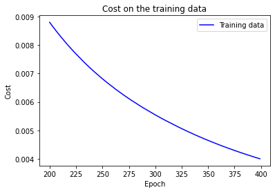
The cost is showing a smooth decrease, approaching zero at the end of 400 epochs. Now let's look at the classification accuracy on the test data over the last 200 epochs:

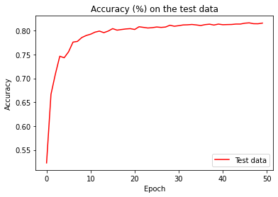
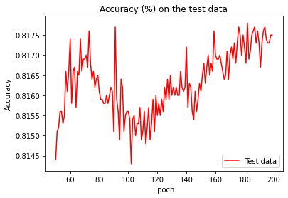
In the first 200 epochs the accuracy rises to just under 82 percent.

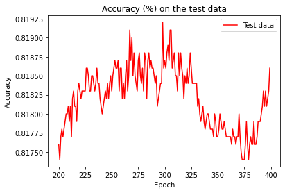
Then the learning gradually slows down. Finally, at around epoch 225 the classification accuracy stops improving. Later epochs merely see small stochastic fluctuations near the previously obtained value at epoch 225. If we look at the graph of cost on the training data, it appears that the network is getting better, while in reality the improvement after epoch 225 is an illusion. We say the network is overfitting beyond epoch 225.

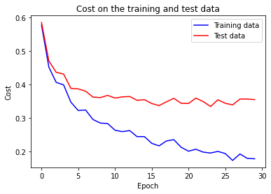
If we compare other criteria, we find the same pattern. For example, the graph of the cost on the test data is the following:

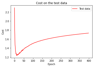
We can see that the cost on the test data improves until around epoch 15, but after that it starts to get worse, even though the cost on the training data is continuing to get better. Should we regard epoch 15 or epoch 225 as the point at which the network no longer generalizes to the test data. In the end what we care is the classification accuracy and the cost is only a proxy to this goal, therefore it makes most sense to regard epoch 225 as the point beyond which overfitting dominates learning in our neural network.

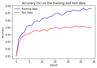
Another sign of overfitting is the graph of classification accuracy on the training data:

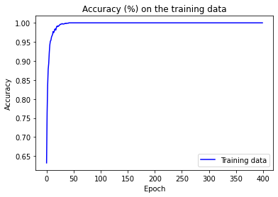
The accuracy rises way up to 100 percent, which means that the network correctly classifies 1,000 training images. At the same time, the test accuracy top at just 81.92 percent. We conclude that the network is merely memorizing the training set without understanding digits well enough to generalize to the test set.

The obvious way to detect overfitting is to keep track of accuracy on the test data as the network trains. If we see that the accuracy on the test data stops improving, we can decide to stop training.

Recall that validation_data contains 10,000 images which are different from training_data. At the end of each epoch we will compute the classification accuracy on the validation_data and when the classification accuracy has saturated, we stop learning. This strategy is call early stopping. In practice, we continue training until we are confident that the accuracy has saturated.

We use validation_data to learn best hyper-parameters such as the learning rate, the number of epochs to train to prevent overfitting, and so on instead of test_data, because we don't want our network to learn these hyper-parameters based on evaluations from the test_data. It is possible that the network will end up overfitting the hyper-parameters to the test_data and fail to generalize for other data sets. After we've got the hyper-parameters we want, we do a final evaluation of accuracy using the test_data. By doing this we can be sure that the results on the test_data are a genuine measure of how well the neural network generalizes. To put it another way, we can think of of the validation_data as a type of training_data that helps us learn good hyper-parameters. This approach is called hold out method, because the validation_data is kept apart from the training_data.

So far we've used 10,000 images to look at overfitting problem. Now what happens if we use the full training set of 50,000 images?

(training_data, validation_data, test_data) = mnist.load_matrix_data()
net3 = network3.Network([784, 30, 10])
net3.large_weight_initializer()
(evaluation_cost,
evaluation_accuracy,
training_cost,
training_accuracy) = net3.SGD(training_data, 30, 10, 0.5,
    evaluation_data=test_data,
    monitor_training_cost=True,
    monitor_training_accuracy=True,
    monitor_evaluation_cost=True,
    monitor_evaluation_accuracy=True)

Now the accuracy on the test and training data is much closer together then when we were using 1,000 training examples. Specifically, the best classification accuracy of 97.73% on the training data is only 2.5 % higher than the 95.2% on the test data. This is in contrast to 18.08% gap we had earlier. The network is generalizing much better with the increased size of the training data. However, training data can be expensive or difficult to acquire, so this is not always practical.

L2 regularization

Increasing the amount of training data is one way of reducing overfitting. Another way is to reduce the size of the network. However, large networks have the potential to be more powerful than small networks. Luckily, there is another method that can reduce overfitting called regularization techniques. One of the most common technique is known as weight decay or L2 regularization. The following is the regularized cross-entropy cost function:

$$ \begin{align} C = -\frac{1}{n} \sum_{xj} \left[ y_j \ln a^L_j+(1-y_j) \ln (1-a^L_j)\right] + \frac{\lambda}{2n} \sum_w w^2. \tag{88} \end{align} $$

The first term is the usual expression for cross-entropy. But we've added the second term, which is sum of the squares of all the weights in the network. This is scaled by a factor $\lambda / 2n$, where $\lambda \gt 0$ is known as the regularization parameter, and $n$ is the size of our training data set. Note that the regularization term does not include the bias for the following reasons:

• having a large bias doesn't make a neuron sensitive to its inputs in the same way as having large weights, so we don't need to worry about large biases enabling our network to learn the noise in the training data;

• allowing large biases gives our network more flexibility in behavior, namely, large biases make it easier for the neurons to saturate, which is sometimes desirable.

It is also possible to regularize other cost functions as well, such as quadratic cost. This is done in a similar way:

$$ \begin{align} C = \frac{1}{2n} \sum_x |y-a^L|^2 + \frac{\lambda}{2n} \sum_w w^2. \tag{89} \end{align} $$

In both cases we can write the regularized cost function as

$$ \begin{align} C = C_0 + \frac{\lambda}{2n} \sum_w w^2, \tag{90} \end{align} $$

where $C_o$ is the original, unregularized cost function.

Intuitively, the effect of regularization is to make the network prefer to learn small weights. Large weights are allowed if they considerably improve the first term of the cost function. We can think of regularization as a compromise between finding small weights and minimizing the original cost function. The relative importance of the compromise depends on the value of $\lambda$: when $\lambda$ is small, we prefer to minimize the original cost function, but when $\lambda$ is large we prefer small weights.

New we need to figure out how to apply stochastic gradient descent learning algorithm in a regularized neural network. We start with computing the partial derivatives $\partial C / \partial w$ and $\partial C / \partial b$ for all the weight and biases in the network:

$$ \begin{align} \frac{\partial C}{\partial w} & = \frac{\partial C_0}{\partial w} + \frac{\lambda}{n} w \tag{91}\\[2ex] \frac{\partial C}{\partial b} & = \frac{\partial C_0}{\partial b}. \tag{92} \end{align} $$

The $\partial C_0 / \partial w$ and $\partial C_0 / \partial b$ terms can be computed using backpropagation. So we can use backpropagation as usual and then add $\frac{\lambda}{n} w$ to the partial derivative of all the weight terms. The partial derivatives with respect to the biases are unchanged, so the gradient descent update rule doesn't change:

$$ \begin{align} b & \rightarrow b -\eta \frac{\partial C_0}{\partial b} \tag{93} \end{align} $$

The learning rule for the weights becomes:

$$ \begin{align} w & \rightarrow w-\eta \frac{\partial C_0}{\partial w}-\frac{\eta \lambda}{n} w \tag{94}\\[2ex] & = \left(1-\frac{\eta \lambda}{n}\right) w -\eta \frac{\partial C_0}{\partial w}. \tag{95} \end{align} $$

This expression is the same as the usual gradient descent learning rule, except we first rescale the weight $w$ by a factor $1-\frac{\eta \lambda}{n}$. This rescaling is sometimes referred as weight decay, because it makes the weights smaller. It seems that this new learning rule will drive the weights toward zero, but it's not the case because the second term may increase the weights if doing so decreases the unregularized cost function.

For the stochastic gradient descent, the regularized learning rule becomes

$$ \begin{align} w & \rightarrow \left(1-\frac{\eta \lambda}{n}\right) w -\frac{\eta}{m} \sum_x \frac{\partial C_x}{\partial w}, \tag{96} \end{align} $$

where the sum is over training examples $x$ in the mini-batch and $C_x$ is the unregularized cost for each training example. Finally, the regularized learning rule for the biases is the same as in the unregularized case:

$$ \begin{align} b & \rightarrow b - \frac{\eta}{m} \sum_x \frac{\partial C_x}{\partial b}, \tag{97} \end{align} $$

where the sum is over training examples $x$ in the mini-batch.

Let's look at the performance of our neural network if we use the regularization parameter $\lambda=0.1$. We will use test_data instead of validation_data to better compare the results with our previous examples. Strictly speaking, we should be using validation_data for the purpose of evaluation of our network performance.

(training_data, validation_data, test_data) = mnist.load_matrix_data()
net3 = network3.Network([784, 30, 10])
net3.large_weight_initializer()
(evaluation_cost,
evaluation_accuracy,
training_cost,
training_accuracy) = net3.SGD((training_data[0][:,:1000],
    training_data[1][:,:1000]), 400, 10, 0.5,
    lmbda = 0.1,
    evaluation_data=test_data,
    monitor_training_cost=True,
    monitor_training_accuracy=True,
    monitor_evaluation_cost=True,
    monitor_evaluation_accuracy=True)

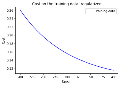
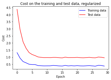
The cost on the training data decreases over the whole time, similar to the unregularized case:

However, this time the accuracy on the test_data continued to increase for the entire 400 epochs:

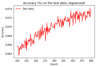
It is clear that the used regularization technique has suppressed overfitting. What's more, the maximum achieved accuracy is 87.42%, which is much higher than 81.92% attained with unregularized network. From our experience we observe that regularization let our neural network to generalize better and reduced the effects of overfitting.

Now let's check the overfitting problem in our network when we feed it with 50,000 training examples. This time though, we need to change the regularization parameter to account for the increased number of training examples which appears in the denominator. If we used the same $\lambda=0.1$, that would mean less decay and accordingly less regularization effect. We compensate by changing to $\lambda=5.0$.

(training_data, validation_data, test_data) = mnist.load_matrix_data()
net3 = network3.Network([784, 30, 10])
net3.large_weight_initializer()
(evaluation_cost,
evaluation_accuracy,
training_cost,
training_accuracy) = net3.SGD(training_data, 30, 10, 0.5,
    lmbda = 5.0,
    evaluation_data=test_data,
    monitor_training_cost=True,
    monitor_training_accuracy=True,
    monitor_evaluation_cost=True,
    monitor_evaluation_accuracy=True)

We get the following results:

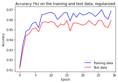
Fist, we observe that our classification accuracy on the test data is up, from 95.20% to 95.95%. Second, the gap between the accuracy metric on the test data and training data is much narrower than before, now running at 1.05% comparing to 2.53% before.

We can explore what test classification accuracy we can get if we use 100 hidden neurons and the regularization parameter $\lambda=5.0$:

(training_data, validation_data, test_data) = mnist.load_matrix_data()
net3 = network3.Network([784, 100, 10])
net3.large_weight_initializer()
(evaluation_cost,
evaluation_accuracy,
training_cost,
training_accuracy) = net3.SGD(training_data, 30, 10, 0.5,
    lmbda = 5.0,
    evaluation_data=test_data,
    monitor_training_cost=True,
    monitor_training_accuracy=True,
    monitor_evaluation_cost=True,
    monitor_evaluation_accuracy=True)

The final result is the classification accuracy of 97.78% on the validation_data. If tune the network a bit more and run it for 60 epochs at $\eta=0.1$ and $\lambda=5.0$, we achieve 98.00% classification accuracy on the validation_data.

Another benefit of regularized network is that it much less likely to get stuck in a local minimum of the cost function whereas unregularized version may sometimes get stuck in it. Therefore the regularized network provides more easily replicable results. This happens because the length of the weight vector is likely to grow large, pointing in more or less the same direction. This phenomenon is making it hard for the learning algorithm to properly explore the weight space.

A regularized network is constrained to build simpler models based on patterns often seen in the training data, and they are resistant to learning peculiarities of the noise in the training data. However, no one has yet developed an entirely convincing theoretical explanation for why regularization helps networks generalize. We don't have an entirely satisfactory systematic understanding of what's going on, merely incomplete heuristics and rules of thumb.

With 100-hidden neurons network we have 79,510 parameters. We have only 50,000 images in our training data so we can easily fit a 79,510 degree polynomial to 50,000 data points, so our network should overfit badly. So why does it generalize? It was conjectured that the dynamics of gradient descent learning in multilayer nets has a self-regularization effect.

L1 regularization

In this technique we modify the unregularized cost function by adding the sum of the absolute values of the weights:

$$ \begin{align} C & = C_0 + \frac{\lambda}{n} \sum_w |w|. \tag{98} \end{align} $$

This is somewhat similar to L2 regularization because we penalize large weights what leads the network to prefer small weights. Following with the analysis, we will try to understand the behavior of L1 regularization method. Differentiating Equation (98), we get:

$$ \begin{align} \frac{\partial C}{\partial w} & = \frac{\partial C_0}{\partial w} + \frac{\lambda}{n} \frac{w}{|w|}. \tag{99} \end{align} $$

Using this expression, we can modify backpropagation to do stochastic gradient descent using L1 regularization. The resulting update rule for an L1 regularized network is

$$ \begin{align} w & \rightarrow w' = \left(1-\frac{\eta \lambda}{n|w|} \right) w - \frac{\eta}{m} \sum_x \frac{\partial C_x}{\partial w}, \tag{100} \end{align} $$

where the sum is over training examples $x$ in the mini-batch and $C_x$ is the unregularized cost for each training example.

In L1 regularization, the weights shrink by a constant amount toward 0. In L2 regularization, the weights shrink by an amount proportional to $w$. Therefore, when a particular weight has a large magnitude $|w|$, L1 regularization shrinks the weight much less than L2 regularization does. Contrary to that, when $|w|$ is small, L1 regularization shrinks the weight much more than L2 regularization. The result is that L1 regularization tends to leave a small number of high importance weight connections, while the other weights are reduced toward zero.

Note that the partial derivative $ \partial C / \partial w$ is not defined when $w=0$, but it doesn't pose a problem for us because we will just apply the unregularized rule for stochastic gradient descent when $w=0$. For this purpose, we use the convention that $\text{sign}(0)=0$ where $\text{sign(w)}=w/|w|$.

Other regularization techniques include dropout and artificially expanding the training data.

Weight initialization

While the cross-entropy cost function helps us to deal with the saturation of neurons in the output layer, it does nothing with the hidden neurons. If any of these neurons are saturated, we are facing a slow learning problem.

Previously we initialized our weights using Gaussian distribution with mean 0 and standard deviation 1. Suppose we have a large input vector with 1,000 neurons, half of which are set to 0, and another half to 1. The result of the weighted output from a single hidden neuron will itself be a Gaussian distribution with mean zero and standard deviation $\sqrt{501}\approx 22.4$, which is broad and not sharply packed. Moreover, it is quite likely that the output activation $\sigma(z)$ from the hidden neuron will be very close to either 1 or 0. This means that the neuron will be saturated. When this happens, making small changes in the weights will make only infinitesimally small changes in the activation of our neuron. That infinitesimally small change in the activation of the hidden neuron will, in turn, barely affect the rest of the neurons in the network, and as a result we will observe only miniscule change in the cost function.

The solution to this problem is to initialize the weights as Gaussian random variables with mean and standard deviation $1/\sqrt{n_{\text in}}$. We will squash the Gaussians down, making it less likely that our neuron will saturate. We will continue to initialize biases as a Gaussian with mean 0 and standard deviation 1.

Let's compare the new method of initializing weights. We do this be removing the line net3.large_weight_initializer() because our network initializes weights using the new method by default.

(training_data, validation_data, test_data) = mnist.load_matrix_data()
net3 = network3.Network([784, 30, 10])
(evaluation_cost,
evaluation_accuracy,
training_cost,
training_accuracy) = net3.SGD(training_data, 30, 10, 0.1,
    lmbda = 5.0,
    evaluation_data=validation_data,
    monitor_evaluation_accuracy=True)

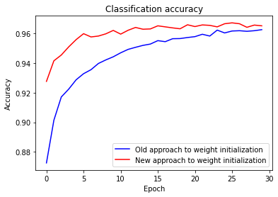
In both cases we end up with a classification accuracy over 96 percent, so the final result is almost the same. But the new initialization technique gets us there much faster. At the end of the first epoch of training the old approach to weight initialization has a classification accuracy of 87.26 percent, while the new approach is already at 92.76 percent. It seems that the new approach to weight initialization starts off in a much better position, which brings us to better results much more quickly. For some neural networks this technique of weight initialization will lead to increase in the speed of learning and final performance.

Adapted from Michael A. Nielsen, "Neural Networks and Deep Learning"