Linear discriminant analysis
Linear discriminant analysis (LDA) is a supervised algorithm that can be used to extract features to increase computational efficiency in non-regularized models. It was first formulated in The Use of Multiple Measurements in Taxonomic Problems by R. A. Fisher in 1936 and then generalized to multi-class problems in The Utilization of Multiple Measurements in Problems of Biological Classification by C. Radhakrishna Rao in 1948.
The concept of LDA is similar to PCA, although it differs slightly. When PCA attempts to find the orthogonal component axes of maximum variance in a dataset, LDA is trying to find feature subspace that optimizes class separability.
We assume that the data is normally distributed, that the classes have identical covariance matrices, and that the training examples are statistically independent of each other.
LDA algorithm
- Standardize the \(d\)-dimensional dataset.
- Compute the \(d\)-dimensional mean vector for each class.
- Construct the between-class scatter matrix \(S_B\) and within-class scatter matrix \(S_W\).
- Compute the eigenvectors and corresponding eigenvalues of the matrix \(S_W^{-1}S_B\).
- Sort the eigenvalues by decreasing order to rank the corresponding eigenvectors.
- Select the \(k\) largest eigenvalues and construct the transformation matrix \(W^{d \times k}\) with eigenvectors in the columns.
- Project the examples onto the new feature subspace using the transformation matrix \(W\).
Scatter matrices
Since we have already standardized the features of the Wine dataset in the PCA part of the article, we can skip the first step and move on with the calculation of the mean vectors, which we will use to construct scatter matrices. Each mean vector \(m_i\) stores the mean feature value with respect to examples of class \(i\):
$$m_i = \frac{1}{n_i} \sum_{x \in D_i}^{n_i} x$$
Using the mean vectors, we can compute the within-class scatter matrix \(S_W\) as a sum of individual scatter matrices of each class \(i\), which we can vectorize (with broadcasting) in matrix form as following:
$$ \begin{align}S_W &= \sum_{i=1}^{c} \sum_{x \in D_i}^{n_i} (x-m_i)(x-m_i)^T\\ &= \sum_{i=1}^{c} (X_i-m_i)^T (X_i-m_i) \end{align}$$
d = X_train_std.shape[1]
S_W = np.zeros((d, d))
mean_vecs = list()

for label in np.unique(y_train):
    A = X_train_std[y_train == label]
    mu = np.mean(A, axis=0) # mean vector per class
    mean_vecs.append(mu)
    S_W += (A - mu).T @ (A - mu)
We assumed that the class labels in the training dataset are uniformly distributed, however it is not the case in our example: there 41 examples in class 1, 50 examples in class 2, and 33 examples in class 3. Therefore, we need to scale the individual scatter matrices \(S_i\) before we sum them up to obtain \(S_W\). This is equivalent to computing the covariance matrix \(\Sigma_i\).
$$ \begin{align}S_W &= \sum_{i=1}^{c} \Sigma_i\\ &= \sum_{i=1}^{c} \frac{1}{n_i-1} S_i\\ &= \sum_{i=1}^{c} \frac{1}{n_i-1} \sum_{x \in D_i}^{n_i} (x-m_i)(x-m_i)^T\\ &= \sum_{i=1}^{c} \frac{1}{n_i-1} (X_i-m_i)^T (X_i-m_i) \end{align}$$
S_W = np.zeros((d, d))

for label, mu in zip(np.unique(y_train), mean_vecs):
    A = X_train_std[y_train == label]
    S_W += ((A - mu).T @ (A - mu))/(A.shape[0]-1)
Now we can proceed to computing the between-class scatter matrix \(S_B\) as the following:
$$ \begin{align}S_B &= \sum_{i=1}^{c} n_i (m_i-m_X)(m_i-m_X)^T\\ \end{align}$$
where \(m_X\) is the overall mean from all examples. Since we have already standardized our data, our overall mean is zero.
mean_overall = np.mean(X_train_std, axis=0)
mean_overall = mean_overall.reshape(d, 1)  # make column vector
S_B = np.zeros((d, d))

for label, mu in zip(np.unique(y_train), mean_vecs):
    A = X_train_std[y_train == label]
    n = A.shape[0]
    mu = mu.reshape(d, 1)  # make column vector
    S_B += n * (mu - mean_overall).dot((mu - mean_overall).T)
Computing linear discriminants
The remaining steps are similar to that of PCA, however this time we solve the eigenvalue problem of the matrix \(S_W^{-1}S_B\). In LDA, the number of linear discriminants is at most \(c-1\), where \(c\) is the number of class labels, since the in-between matrix \(S_B\) is the sum of \(c\) matrices with rank one or less.
eigen_vals, eigen_vecs = np.linalg.eig(np.linalg.inv(S_W) @ S_B)
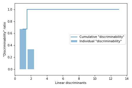
Next we will calculate the "discriminability" ratios and plot the cumulative sum of discriminabilities on the Scree plot to view the contribution of each linear discriminant to the variance in the data.
eigen_vals_tot = np.sum(eigen_vals.real)
discr = [(i / eigen_vals_tot) for i in sorted(eigen_vals.real, reverse=True)]
cum_discr = np.cumsum(discr)
Feature transformation
At this final step we need to sort the eigenvalues by decreasing order to rank the corresponding eigenvectors and then create the transformation matrix \(W\) by putting two most important eigenvectors as column vectors.
eigen_pairs = [(np.abs(eigen_vals[i]), eigen_vecs[:, i])
               for i in range(len(eigen_vals))]

eigen_pairs.sort(key=lambda k: k[0], reverse=True)

W = np.vstack((eigen_pairs[0][1].real, eigen_pairs[1][1].real)).T
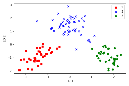
Using the transformation matrix \(W\), we can now transform the training dataset.
$$X' = XW$$
X_train_lda = X_train_std @ W
We can see that the three Wine classes could be linearly separated in the new feature subspace.
LDA in scikit-learn
After we figured out all ins and outs of LDA, we can use scikit-learn library to implement LDA easily.
from sklearn.discriminant_analysis import LinearDiscriminantAnalysis as LDA

lda = LDA(n_components=2)
X_train_lda = lda.fit_transform(X_train_std, y_train)
X_test_lda = lda.transform(X_test_std)
We will train a simple logistic regression model on the lower-dimensional data and check how it performs with generalization on unseen test data.
from sklearn.linear_model import LogisticRegression

lr = LogisticRegression(multi_class='ovr', random_state=1, solver='lbfgs')
lr = lr.fit(X_train_lda, y_train)
test_score = np.sum(lr.predict(X_test_lda) == y_test)/y_test.shape[0]
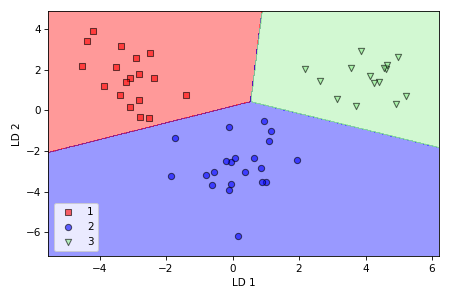
We can see from decision regions plot that logistic regression performed well on novel data, separating the three classes with 100% accuracy.
The supporting code for this article is available on Github.
Adapted from Sebastian Raschka & Vahid Mirjalili, "Python Machine Learning".