Statistical machine learning framework

Notation

Linear Algebra and Matrix Notation

$$\begin{array}{ll} f: D \to R &\text{Function on domain $D$ with range $R$}\\ \text{$a$ or $A$} &\text{Scalar variable}\\ \boldsymbol{a} &\text{Column vector (lowercase boldface)}\\ \boldsymbol{a}^T &\text{Transpose of a column vector $\boldsymbol{a}$}\\ \boldsymbol{\ddot a} &\text{$\boldsymbol{\ddot a}: D \to R$ is an approximation for $\boldsymbol{a}: D \to R$}\\ \end{array}$$

Random Variables

$$\begin{array}{ll} \tilde a\phantom{: D \to R} &\text{Scalar random variable}\\ \boldsymbol{\tilde a} &\text{Random column vector}\\ \boldsymbol{\tilde A} &\text{Random matrix}\\ \hat a &\text{Random scalar-valued function}\\ \boldsymbol{\hat a} &\text{Random vector-valued function}\\ \mathcal{B}^d &\text{Borel sigma-field generated by open sets in $\mathcal{R}^d$}\\ \end{array}$$

Probability Theory and Information Theory

Special Functions and Symbols

Machine learning environments

Deductive inference machines generate logical inferences from input patterns using a knowledge base which is a set of rules. Inductive inference machines generate plausible inferences from input patterns using a knowledge base which is a collection of beliefs.

Training data is assumed to be generated from the environment by sampling from a probability distribution called the environmental distribution. The process that generates the training data is called the data generating process. The knowledge base of a statistical learning machine is a set of probability distributions (called the probability model). Specific beliefs may reflect the relevance of the probability model to approximate the environmental distribution.

The goal of the machine learning process is to search for the probability distribution in the probability model which best approximates the environmental distribution. The machine then uses this best-approximating distribution to make probabilistic inductive inferences.

Feature vectors

A feature map is a function that maps an environmental event into a feature vector whose elements are real numbers. An environmental event may be the air pressure generated by a human voice or the behavior of the stock market. The feature vector suppresses irrelevant information and exaggerates relevant information in order to provide an appropriate abstract representation of the event.

A numerical coding scheme is used to model the output of a collection of sensors, such as the output voltage of a microphone at a particular time or the closing price of a security on a particular day.

A binary coding scheme is used to model the presence or attribute of a feature. A present-absent binary coding scheme corresponds to a feature map that returns the value one if some environmental event is present, and zero if it is absent. A present-unobservable binary scheme returns one if the event is present and zero if the event is unobservable.

A categorical coding scheme models an $M$-valued categorical variable. One-hot encoding scheme represents a categorical variable $M$ such that $k$th value is an M-dimensional vector with a one in its $k$th position and zeros in the remaining elements of the vector. Reference cell coding encodes an $M$-valued categorical variable as an $M-1$-dimensional vector such that $M-1$ values are represented as an identity matrix and the last value is represented as a zero vector.

The curse of dimensionality, first introduced by Bellman in 1961, underlines the fact that the more features we have as the input, the more difficult it becomes to solve the problem, even though with increased number of features we have a larger space to look for the best approximation of the environmental distribution. For example, if we have $M$ possible values of each feature, $d$ features, and a binary classification output (zero and one), we would have $M^d$ possible input patterns and $2M^d$ possible input-to-output mappings. The number of samples needed to estimate an arbitrary function with a given level of accuracy grows exponentially with respect to the number of input variables (i.e., dimensionality) of the function.

In order to reduce feature vector dimensionality, the solution is to choose a good subset of all possible input features that will improve the performance of the learning machine. The problem of selecting the best subset of features is called best subsets regression (Beale et al. 1967; Miller 2002). Dong and Liu (2018) provide a modern review of feature engineering methods for machine learning.

Stationary environments

It is typical to assume that the statistical environment is stationary which implies that there are statistical regularities in the training data that can be useful to process the novel test data. However, the environment may change, and the old training data may no longer represent the new data (consider a model trained on the data collected while the economy had low inflation to make predictions when the economy has high inflation). For some applications machine learning environment is either stationary, slowing changing, or a sequence of environments that converges to a stationary environment.

Strategies for machine learning algorithms

In adaptive learning the machine updates its current knowledge each time it is faced with a new event in a sequence. In batch learning the machine updates its current state of knowledge after it looks through the entire collection of events. With minibatch learning the machine updates its current state each time a subset of events is experienced. Batch learning is preferred, however it could be too computationally intensive or parts of the data set are only incrementally available over time.

In reactive environment reinforcement learning the machine interacts with its environment during the learning process and updates its knowledge based on its actions and feedback from the environment (consider learning to land a helicopter in the presence of violent wind gusts). Some research is focused on teaching learning machines through the construction of a sequence of stationary environments (Konidaris and Barto 2006; Pan and Yang 2010; Taylor and Stone 2009; Bengio et al. 2009).

Prior knowledge

A large data set does not necessarily imply that the data set contains sufficient information to produce reliable inferences (consider guessing a name of people based on their age). Prior environmental knowledge can set specific hints and constraints that will improve generalization performance.

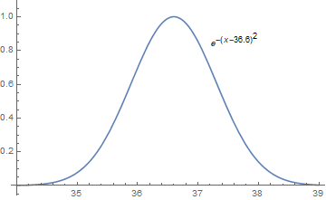
A poorly chosen feature vector can impede the learning process. For example, if we calculate the health score based on the patient's temperature $s$ as $f(s) = s - \beta$, then we cannot find a proper $\beta$ such that the patient will be assigned a small health score if the temperature is much larger or much smaller than $36.6$. On the other hand, if we set $f(s) = e^{-(s-\beta)^2}$, then it is easy to give a health score by detecting abnormal body temperatures.

Health score

Another idea how prior knowledge can improve inference is the assumption that similar input patterns should generate similar responses. For example, if we have $d$ binary inputs, then it is possible to represent $2^d$ possible $d$-dimensional binary input pattern vectors. If we make an inference of the probability that the response variable takes on the value of one for each of the possible $2^d$ input patterns with $2^d$ free parameters in the model, this model does not include prior knowledge and is called the contingency table model. In contrast, logistic regression model estimates a weighted sum of the $d$ binary input variables with $d$ weights as free parameters instead of $2^d$ as in the previous case. This exponential reduction increases speed of learning and includes prior knowledge about similar input patterns. However, in environments where such assumption fails, logistic regression may exhibit severe difficulties in learning due to a much smaller range of probability distributions when compared with the contingency table representation scheme.

Regularization also incorporates prior knowledge by treating many of its free parameters as irrelevant. Convolutional neural networks (CNNs) incorporate prior knowledge by learning statistical regularities of an image that are not location-specific within the image. Recurrent neural networks (RNNs) use parameter sharing for learning time-invariant statistical regularities. Goodfellow et al. (2016) provides a comprehensive introduction to the CNNs and RNNs, and Schmidhuber (2015) provides a recent review of the literature.

Empirical risk minimization

Artificial neural network node

The architecture of machine learning algorithms was first introduced in the Artificial Neural Network (ANN) literature (Rosenblatt 1962; Rumelhart, Hinton, and McClelland 1986). This ANN graphical notation depicts a learning algorithm as a collection of nodes or units where each node has a state called its activity level, which is typically a real number. An output unit produces its activity level from the activity level of the input units, weighted by the unit-specific set of parameters, which are called the connection weights for the unit. Such a formulation of state-updating and learning dynamics corresponds to a dynamical system specification of the machine learning algorithm.

Artificial Neural Network node

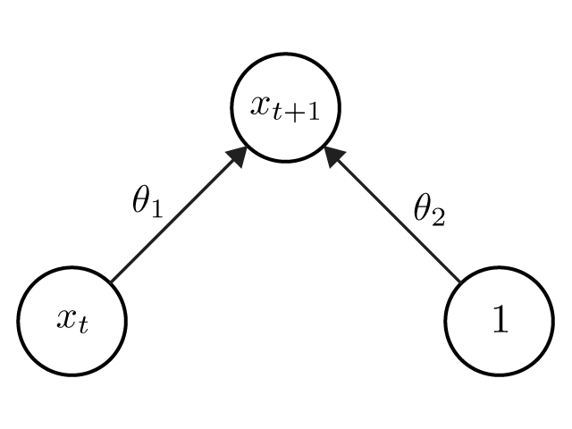
For example, in the picture the input has two nodes whose states are $x_t$ and $1$. The output is the prediction of state $x_{t+1}$ which is computed as the weighted sum of states of the two input patterns: $\hat x_{t+1} (\theta) = \theta_1 x_t + \theta_2$.

Risk functions

In empirical risk minimization (ERM) problem we assume that there is a data distribution $P$ in the statistical environment which is unknown to us. We would like to know how well a learning machine will work in practice by minimizing the true risk. However, the machine has detected only $n$ environmental events as a collection of $d$-dimensional feature vectors or training vectors from that data distribution. Therefore the next best thing we can do instead is minimize the expected risk over the empirical distribution of the observed data.

The set of $n$ training vectors $\boldsymbol{x_1}, \ldots, \boldsymbol{x_n}$ is called the training data set $\mathcal{D} _ n$. The machine's state of knowledge is specified by a parameter vector $\boldsymbol{\theta}$. The goal of the learning process is to choose the best values of $\boldsymbol{\theta}$.

The learning machine's actions and decisions are entirely determined by the parameter vector $\boldsymbol{\theta}$. Let $\boldsymbol{x} \in \mathcal{D} _ n$ denote a training vector. The quality of the learning machine's ability to make good actions and decisions when the machine observes $\boldsymbol{x}$ with a current parameter vector $\boldsymbol{\theta}$ is measured by a loss function $c$ which maps $\boldsymbol{x}$ and $\boldsymbol{\theta}$ into a real number $c(\boldsymbol{x, \theta})$, which is interpreted as a penalty given to the machine for experiencing the event vector $\boldsymbol{x}$. In order to minimize the penalty, the machine is searching for a parameter vector $\boldsymbol{\theta}$ that minimizes the empirical risk function (expected risk over empirical distribution)

$$\mathscr{\hat l_n} (\boldsymbol{\theta}) = \frac 1n \sum_{i=1}^n c(\boldsymbol{x} _ i,\boldsymbol{\theta})$$

where the set $\mathcal{D} _ n \equiv [\boldsymbol{x_1}, \ldots, \boldsymbol{x_n}]$ is the training data.

Since the machine has observed only a limited number of samples $n$, the empirical distribution may not represent the distribution $P$ well enough. However, by the Glivenko–Cantelli theorem, the empirical distribution converges uniformly to the population distribution almost surely as $n$ increases.

If we assume that the test data set is drawn from the same distribution $P$ as the training data (which is often not the case), then the empirical risk on the test data will be a better estimate of the true risk than the empirical risk computed on the training data, because the learning machine can potentially overfit to the latter.

Example 1. Suppose we have a binary classification machine learning problem. Let $p(y=1|s)$ denote the probability that a learning machine believes the response category $y=1$ is correct given input pattern $s$.

The minimum probability decision rule is to choose $y=1$ when $p(y=1|s) > p(y=0|s)$ and choose $y=0$ otherwise. We can rewrite the minimum probability or error decision rule as:

$$p(y=1|s) > 1 - p(y=1|s)$$

which in turn we can rewrite as $p(y=1|s) > 0.5$. Therefore, we choose the response category $y=1$ when $p(y=1|s) > 0.5$ and we choose the response category $y=0$ when $p(y=1|s) < 0.5$. The probability that a particular response is correct is given by the formula:

$$p(y|s) = yp(y=1|s) + (1-y)(1-p(y=1|s))$$

Example 2. Suppose we denote a closing price of a security at day $t$ as $x_t$ and parameter vector $\theta=(\theta_1, \theta_2)$ to predict $x_{t+1}$. Let the closing price prediction be expressed by the formula:

$$\hat x_{t+1} (\theta) = \theta_1 x_t + \theta_2$$

Assume we have a history of closing prices for the security over the past $n$ days denoted by $x_1, x_2, \ldots, x_n$. The machine's performance is measured by the empirical risk function:

$$\mathscr{\hat l_n} (\theta) = \frac 1{n-1} \sum_{t=1}^{n-1} C([x_t,x_{t+1}],\theta)$$

The loss function is defined as the least squares:

$$C([x_t,x_{t+1}],\theta) = (x_{t+1} - \hat x_{t+1} (\theta))^2$$

After substituting the loss function into the empirical risk function we get:

$$\mathscr{\hat l_n} (\theta) = \frac 1{n-1} \sum_{t=1}^{n-1} (x_{t+1} - \theta_1 x_t - \theta_2)^2$$

Regularization terms

A regularization term $k_n (\theta)$ penalizes non-sparse choices of parameter vector $\theta$, and takes on a smaller value if the values of $\theta$ are close to zero, which corresponds to a sparse solution. Sparse solutions help reduce overfitting because non-sparse solutions learn random noise which is usually not present in the test data. The regularization term is added to the empirical risk function as following:

$$\mathscr{\hat l_n} (\theta) = \frac 1n \sum_{i=1}^n C(x_i,\theta) + k_n (\theta).$$

Let $\lambda$ be a positive real number and $\theta = [\theta_1, \ldots, \theta_q]^T$. A regularization term

$$k_n (\theta) = \lambda |\theta|^2$$

where $|\theta|^2 = \sum_{j=1}^q \theta_j^2$ is called $L_2$ or ridge regression regularization term. A regularization term

$$k_n (\theta) = \lambda |\theta|_1$$

where $|\theta| 1 = \sum{j=1}^q |\theta_j|$ is called $L_1$ or lasso regularization term. A regularization term

$$k_n (\theta) = \lambda |\theta|^2 + (1-\lambda) |\theta|_1, \quad 0 \le \lambda \le 1$$

is called an elastic net regularization term.

The objective function should be differentiable, however $L_1$ regularization term is not differentiable. We can either smooth it with an approximation

$$|\theta_j| \approx ((\theta_j)^2 + \epsilon^2)^{\frac 12}$$

where $\epsilon$ is a small positive real number such that $|\theta_j| \lt \lt \epsilon$. Or we can use the another approximation:

$$|\theta_j| \approx \tau \mathcal{J} (\theta_j/\tau) + \tau \mathcal{J} (-\theta_j/\tau)$$

where $\mathcal{J}(\phi) \equiv \log(1+e^{\phi})$ and $\tau$ is a sufficiently small positive number.

Optimization methods

The objective of the learning algorithm is to find the optimal parameters $\theta$ that minimize the empirical risk function $\mathscr{\hat l_n} (\theta)$. The main idea of optimization methods is to start with an initial guess denoted by $\theta (0)$ and then for $t=0,1,2,\ldots$, refine this initial guess so that the refined guess has a smaller empirical risk $\mathscr{\hat l_n} (\theta(t+1))$.

Many of batch machine learning algorithms have a single type of iterative algorithm at its core. This algorithms is call the method of gradient descent. We denote

$$\frac{d\mathscr{\hat l_n} (\theta(t))}{d\theta}$$

to be the gradient of $\mathscr{\hat l_n}$ evaluated at $\theta(t)$. The iterative formula of gradient descent is the following:

$$\theta(t+1) = \theta(t) - \eta_t \frac{d\mathscr{\hat l_n} (\theta(t))}{d\theta}$$

where $\eta_t$ is a postivie real number called the learning rate. By applying the iterative formula of gradient descent again we can get the refined estimate $\theta(t+2)$, and so on until we converge to the desirable minimum of $\mathscr{\hat l_n}$. Variations of the gradient descent iterative algorithm include Levenberg-Marquardt and L-BFGS algorithms that converge faster.

One method of deciding when to stop the iteration is to check if $\theta (t+1) \approx \theta (t)$. Another consideration is to check the magnitude of the derivative of $\mathscr{\hat l_n}$ is small enough.

Recall the empirical risk function is defined as

$$\mathscr{\hat l_n} (\theta) = \frac 1n \sum_{i=1}^n C(x_i,\theta)$$

In statistical environments where only a small amount of training data becomes incrementally available to the learning machine, we use adaptive gradient descent which updates the parameters $\theta$ ones per each training example instead of going through the whole batch of training data with the empirical risk function substituted by the loss function:

$$\theta(t+1) = \theta(t) - \eta_t \frac{dC(x_i,\theta(t))}{d\theta}$$

Example 3 (example 2 continued). Design a batch gradient descent algorithm for stock market prediction. We calculate the gradient of the loss function with respect to the parameter vector as following:

$$ \begin{align} \nabla_{\theta} C(\theta) & = \left[ \begin{array}{c} \frac{\partial C(\theta)}{\partial \theta_1} \\ \frac{\partial C(\theta)}{\partial \theta_2} \\ \end{array} \right], \quad \theta \in \mathbb{R}^{n} \\[2ex] \nabla_{\theta} C(\theta) & = \left[ \begin{array}{c} -2x_t(x_{t+1} - \theta_1 x_t - \theta_2) \\ -2(x_{t+1} - \theta_1 x_t - \theta_2) \\ \end{array} \right] \end{align} $$

Substituting the gradient of the loss function into the gradient descent learning rule formula, we get

$$ \begin{align} \theta_1 (k+1) & = \theta_1(k) + \frac{2\eta_k}{n-1} \sum_{t=1}^{n-1} x_t(x_{t+1} - \theta_1 x_t - \theta_2)\\ \theta_2 (k+1) & = \theta_2(k) + \frac{2\eta_k}{n-1} \sum_{t=1}^{n-1} (x_{t+1} - \theta_1 x_t - \theta_2) \end{align} $$

where $\eta_1, \eta_2, \ldots$ is a sequence of learning rates.

Machine learning algorithm design

Stage 1: System specification

The inference and learning algorithm is mathematically specified as a dynamical system whose goal is to minimize an objective function. The specification should include a careful analysis of the structural features of the environment. The mathematical specification consists of two parts: (i) optimization algorithm and (ii) objective function.

Step 1: Specify learning machine's statistical environment. What are the environmental events? How to represent events as feature vectors? Is the environment stationary?

Step 2: Specify machine learning architecture. Select a parametric form that provide hints about structure of the environment. Begin with the simplest architecture capable of solving the problem, understand it, and move to more complicated architectures. Add regularization terms if necessary.

Step 3: Specify loss function. Choose a differentiable loss function for empirical risk function that incorporates prior knowledge about the problem.

Step 4: Design inference and learning algorithms. Take the gradient of the loss function to design inference and learning algorithms.

Stage 2: Theoretical analyses

Investigate the conditions which ensure that the machine generates a sequence of parameter updates that converge to a desirable knowledge state. Analysis should be performed on the machine's generalization performance on the new data.

Step 5: Design evaluative methods for analyzing performance. Use the gradient of the loss function to design performance evaluation methods.

Stage 3: Physical implementation

Implement the system with software or hardware using the specification designed at the stage 1. Stage 2 provides theorems which describes asymptotic behavior.

Step 6: Implement algorithm and evaluation methods in software. Verify that the implementation follows the documented specification (step 2 and 3) and evaluation methods (step 5).

Stage 4: System behavior evaluation

The performance of the physical system developed in stage 3 is compared with respect to the theoretical predictions of stage 2. It it fails to perform as predicted, then it should be checked to reflect algorithm specifications in stage 1. The assumptions and predictions of stage 2 can be re-evaluated in order to revise algorithm specifications in stage 1.

Step 7: Evaluate algorithm's behavior.

Step 8: Repeat the process until satisfactory performance is achieved.

Supervised learning machines

Discrepancy functions

The training vector $x \equiv (s,y)$ in a supervised problem is represented as a pair of an input pattern vector $s$ and the desired response vector $y$. The loss function $C$ for the ERF has the following form:

$$C(x,\theta) = D(y,\hat y(s,\theta))$$

where $D$ is called the discrepancy function which compares the desired response $y$ to the predicted response $\hat y(s,\theta)$ for a given input pattern $s$ and a given parameter vector $\theta$ (knowledge state). The loss function implicitly incorporates prior knowledge about statistical regularities in the training data and what types of solutions to minimize empirical risk function are better.

A generic adaptive gradient descent supervised learning algorithm (1) is the following:

procedure Supervised-Learning-Gradient-Descent(theta(0))
    t = 0
    repeat
        Select next training example x(t)
        g(x(t),theta(t)) = dC(x(t),theta(t))/dtheta
        theta(t+1) = theta(t) - eta*g(x(t),theta(t))
        t = t+1
    until Abs(theta(t) - theta(t+1)) < epsilon
    return {theta(t)}
end procedure

Linear regression

A linear regression or least squares discrepancy measure is most appropriate when the response $y$ is a continuous numerical quantity. We define the predicted response as

$$\hat y(s,\theta) = \theta^T[s^T \quad 1]^T$$

We choose the discrepancy function as following:

$$ D(y,\hat y(s,\theta)) = (y - \hat y(s,\theta))^2$$

The empirical risk function is defined for the training set $\mathcal{D}_ n = \{(s_1, y_1), \ldots, (s_n, y_n)\}$ such that

$$\mathscr{\hat l_n} (\theta) = \frac 1n \sum_{i=1}^n (y - \hat y(s,\theta))^2$$

The parameters $\theta$ of the linear regression model are estimated using the algorithm (1).

Logistic regression

A logistic regression discrepancy measure is most appropriate in situations where the desired response is binary-valued. In this case, the machine estimates the probability $p(y=1)$ for a given input pattern $s$ and parameter $\theta$ as the following:

$$p(s,\theta) = \frac{1}{1+e^{-\hat y(s,\theta)}}$$

We choose the discrepancy function $D$ such that:

$$D(y,\hat y) = -[y \log(p(s,\theta)) + (1-y) \log(1-p(s,\theta))]$$

With this choice of discrepancy function, the empirical risk function is defined as following:

$$\mathscr{\hat l_n} (\theta) = -\frac 1n \sum_{i=1}^n [y_i \log(p(s_i,\theta)) + (1-y_i) \log(1-p(s_i,\theta))]$$

Multinomial logistic regression

A multinomial logistic regression or softmax discrepancy measure is appropriate when the desired response is a multi-categorical variable. It is a generalization of the logistic regression discrepancy measure.

We are going to use one-hot encoding for the categorical desired response variable, such that $y^k$ is an $m$-dimensional vector of zeros except for the $k$th component, which has the value of one:

$$y^{k=2} = \left[ \begin{array}{c} 0 \\ 1 \\ 0 \\ 0 \\ \vdots \\ \end{array} \right]$$

Let the parameter matrix $W$ has $m$ rows and $d$ columns:

$$W^{m \times d} = \left[ \begin{array}{cc} W_{11} & W_{12} & \ldots & W_{1d} \\ W_{21} & W_{22} & \ldots & W_{2d} \\ \vdots & \vdots & \vdots & \vdots \\ W_{m1} & W_{m2} & \ldots & W_{md} \\ \end{array} \right]$$

Let $1_m$ be an $m$-dimensional column vector of ones:

$$1_m = \left[ \begin{array}{c} 1 \\ 1 \\ \vdots \\ 1 \\ \end{array} \right]$$

Let $\psi(s;W) = Ws$ and $\psi_k(s;W)$ denote the $k$th element of $\psi(s;W)$ for $k=1, \ldots, m$. The probability that the input vector $s$ is assigned to the $k$th out of $m$ possible categories is the following:

$$p(y_i^k|s_i;W) = \frac{e^{\psi_k(s_i;W)}}{1_m^T e^{\psi(s_i;W)}}$$

We choose the discrepancy function to be the minus natural logarithm of the probability:

$$D(y,s;W) = -y^T\log(p(s;W))$$

Having chosen the discrepancy function, the empirical risk function is the following:

$$\mathscr{\hat l_n} (\theta) = -\frac 1n \sum_{i=1}^n y_i^T\log(p(s_i;W))$$

Basis functions and hidden units

We cannot assume that the predicted response function $\hat y(s,\theta)$ is a weighted sum of the elements of the input pattern vector $s$ when the predicted response is a nonlinear function of $s$ and $\theta$. If we have a hidden layer that is sandwiched between the input pattern layer and the output layer, the predicted response is the following:

$$\hat y(s,\theta) = \sum_{j=1}^J w_j h_j (s,v_j)$$

where the parameter vector $\theta$ concatenates two parameter vectors $w$ and $v$. The basis functions or the hidden units $h_1, h_2, \ldots, h_j$ specify a transformation of $s$ into a new feature vector $h$ which, combined with parameter vector $w$, may be represented as a linear transformation of $h$ to the predicted response $\hat y(s,\theta)$.

The network that has one layer of hidden units is called a multilayer perceptron or shallow neural network. When the inputs of the $k$th layer are functionally dependent on the outputs from $(k-1)$th layer of hidden units, this network architecture is called feedforward network. A network with two or more hidden layers is called a deep learning network.

The number of hidden units defines the information bottleneck that forces the network to extract the most important statistical regularities in its environment and prevents the system from memorizing random noise. Choosing too many hidden units results in memorizing the training dataset, while choosing two few prevents the network from being able to extract the most important patterns.

We can view a nonlinear transformation from the input pattern vector to the hidden unit vector as recording information about the environment. The state activation pattern that is produced by the hidden layer is called an embedding feature representation, and the learnable nonlinear transformation from input pattern to the embedding feature representation is called an embedding layer.

We can use a shallow neural network to approximate any arbitrary continuous function (Hornik 1991; Pinkus 1999) and it can be shown that multilayer perceptrons with two hidden layers are capable of approximating an arbitrary continuous function with a finite number of hidden units (Guliyev and Ismailov 2018).

It is important to initialize the parameter values of the hidden units with small zero-mean random values because this way we allow different hidden units to learn to detect different types of patterns (Sutsekevar et al. 2013).

Multilayer perceptron

Let $y$ denote the desired response (target) of the learning machine given input pattern $s$.

$$s = \left[ \begin{array}{c} s_1 \\ s_2 \\ \vdots \\ s_d \\ \end{array} \right]$$

Let $\hat y(s,\theta)$ denote the predicted response given the input pattern $s$ and parameter vector $\theta$. The goal of the learning process is to find a particular parameter vector $\theta$ such that $\hat y \approx y$ for a given input pattern $s$. Let $h(z)$ be a vector-valued basis function which produces the vector $[h_1, \ldots, h_m]$ of hidden units $h_j$ that maps a subset of the elements of $s$ and $\theta$ into a real number $h_j(s,\theta)$. The predicted response is computed the following way:

$$\hat y(s,\theta) = Vh(s,W)$$

where $W$ is a matrix that specifies the parameters from the input units to the hidden units:

$$Ws = \left[ \begin{array}{cc} W_{11} & W_{12} & \ldots & W_{1d} \\ W_{21} & W_{22} & \ldots & W_{2d} \\ \vdots & \vdots & \vdots & \vdots \\ W_{m1} & W_{m2} & \ldots & W_{md} \\ \end{array} \right] \left[ \begin{array}{c} s_1 \\ s_2 \\ \vdots \\ s_d \\ \end{array} \right] = \left[ \begin{array}{c} \sum_{i=1}^{d}W_{1i}s_i \\ \sum_{i=1}^{d}W_{2i}s_i \\ \vdots \\ \sum_{i=1}^{d}W_{mi}s_i \\ \end{array} \right]$$

the results of which is then fed into the basis function $h$:

$$h(s,W) = h\left( \left[ \begin{array}{c} \sum_{i=1}^{d}W_{1i}s_i \\ \sum_{i=1}^{d}W_{2i}s_i \\ \vdots \\ \sum_{i=1}^{d}W_{mi}s_i \\ \end{array} \right] \right) = \left[ \begin{array}{c} h_1 \\ h_2 \\ \vdots \\ h_m \\ \end{array} \right]$$

and $V$ is a matrix that specifies the connection values from the hidden units to the output units:

$$V^{p \times m} = \left[ \begin{array}{cc} V_{11} & V_{12} & \ldots & V_{1m} \\ V_{21} & V_{22} & \ldots & V_{2m} \\ \vdots & \vdots & \vdots & \vdots \\ V_{p1} & V_{p2} & \ldots & V_{pm} \\ \end{array} \right]$$

$$V h(W,s) = \left[ \begin{array}{cc} V_{11} & V_{12} & \ldots & V_{1m} \\ V_{21} & V_{22} & \ldots & V_{2m} \\ \vdots & \vdots & \vdots & \vdots \\ V_{p1} & V_{p2} & \ldots & V_{pm} \\ \end{array} \right] \left[ \begin{array}{c} h_1 \\ h_2 \\ \vdots \\ h_m \\ \end{array} \right] = \left[ \begin{array}{c} \sum_{i=1}^{m}V_{1i}h_i \\ \sum_{i=1}^{m}V_{2i}h_i \\ \vdots \\ \sum_{i=1}^{m}V_{pi}h_i \\ \end{array} \right]$$

Note that $\theta$ is the concatenation of matrices $W$ and $V$.

Residual network multilayer perceptron

Residual net feedforward perceptron with skip connections build upon the basic multilayer perceptron model by introducing a skip layer $Q$ that connects the input units to the output units directly:

$$\hat y(s,\theta) = Vh(s,W) + Qs$$

The parameter vector $\theta$ consists of the elements of $W$, $V$, and $Q$. The idea of residual network is that linear mapping can be learned to find a linear solution. If the linear solution is not appropriate, then the parameters $W$ and $V$ compensate by using nonlinearities. This skip connections can be interpreted as regularization that introduces smoothness constraints on the objective function (Orhan and Pitkow 2018)

Radial basis functions

There are many choices to choose the basis function from. One of them is the Radial basis function (RBF) defined as:

$$h_j (s,\theta) = G(s-\theta_j)$$

where $G(x)$ is called a Gaussian radial function centered at $\theta_j$ with radius $\sigma$:

$$G(x) = \exp(-\frac{x^T x}{2\sigma^2})$$

A radial basis function has large response signal for $s$ centered at $\theta_j$ and small values elsewhere. It looks like a Gaussian function $g(x) = \frac{1}{\sigma\sqrt{2\pi}} \exp(\frac{-(x-\mu)^2}{2\sigma^2})$ but is not normalized (does not integrate to one). The weighted sum of the output values of the radial basis functions can approximate any arbitrary smooth function.

Sigmoid basis functions

Sigmoid basis functions are defined as

$$h_j (s,\theta) = \mathcal{S} \left( \frac{\theta_j^T s}{\tau} \right)$$

where $\tau$ is a positive number and the logistic sigmoid function is defined as

$$\mathcal{S} (\phi) = \frac{1}{1+\exp(-\phi)}$$

The weighted sum $\mathcal{S}(\phi) - \mathcal{S}(\phi - b)$ models a bump of width $b$, just like radial basis functions. Additionally, the sigmoid basis functions in multilayer perceptrons can be interpreted as incorporating different logistic regression models. Logistic sigmoid function can also be used to construct any AND, OR, and NOT logic gates by manipulating the parameter values $\theta$, which are the building blocks of the modern computer (McCulloch and Pitts 1943).

Another choice for sigmoid function is the hyperbolic tangent sigmoid function defined as:

$$h_j (s,\theta) = 2 \mathcal{S} \left( 2 \theta_j^T s - 1 \right)$$

Softplus basis functions

Softplus basis functions are superior to sigmoid basis functions in deep neural networks. A softplus function $\mathcal{J}$ is defined as:

$$\mathcal{J} (\phi) = \log (1 + \exp(\phi))$$

Likewise, the weighted sum of $\mathcal{J} (\theta) - \mathcal{J} (\theta - b)$ can approximate any nonlinear function.

The formula for the softplus basis function is the following:

$$h_j (s,\theta) = \tau \mathcal{J} (\frac{\phi_j}{\tau})$$

where $\tau$ is a small positive number and $\phi_j \equiv \theta_j^T s$. As $\tau \to 0$, the softplus function converges to a rectlinear basis function which returns $\phi_j$ when $\tau \gt 0$ and returns zero otherwise.

Recurrent neural networks

In some situations we are faced with a problem of identifying patterns in a sequence of data over space or time. We assume that the statistical environment generates a sequence of distributed episodes as a sequence of state vectors $ x_i = (s_i(1),y_i(1)), \ldots, (s_i(T_i),y_i(T_i))$ of length $T_i$ which are highly correlated. $s_i(t)$ corresponds to the $t$th pattern observed in the $i$th episode, and $y_i(t)$ is the response of the learning machine which depends on both the current input pattern $s_i(t)$ as well as on the history of observations within the current episode $(s_i(1),y_i(1)), \ldots, (s_i(t-1),y_i(t-1))$. In general, the desired response $y_i(t)$ specifies the $k$th category of $m$ possible categories by the $k$th column of an $m$-dimensional identity matrix.

The applications of RNN include:

Sequence prediction: predict the next event in the sequence after observing an ordered sequence in an episode.
Sequence classification: predict the class of the sequence after observing an ordered sequence in an episode.
Sequence generation: generate an ordered sequence of responses $y_i(1), \ldots, y_i(T_i)$ given an input pattern $s_i(1)$ for the $i$th episode. In this case, the input pattern sequence is a sequence of the same vectors, which is the context vector of the $i$th episode.
Sequence translation: generate a response $y_i(t)$ for a given input pattern $s_i(t)$, taking into account the temporal context for $s_i$ which includes previous history of input patterns and the past history of desired responses.

Simple recurrent neural network

The key ideas of RNN can be easily understood by a simple recurrent Elman neural network (Elman 1990 and Elman 1991). Let the desired response vector $y_i(t)$ specifies the $k$th out of $m$ possible categories when $y_i(t)$ is equal to the $k$th column of an $m$-dimensional identity matrix:

$$y^{k=2} = \left[ \begin{array}{c} 0 \\ 1 \\ 0 \\ 0 \\ \vdots \\ \end{array} \right]$$

Let the predicted response be a softmax response function:

$$\hat y_i(t) = \frac{\exp(\psi_i(t))}{1_m^T \exp(\psi_i(t))}, \quad \psi_i(t) \equiv Wh_i(t)$$

where $1_m$ is an $m$-dimensional vector of ones and the $k$th element of $\hat y_i(t)$ is the predicted probability that the input pattern vector $s_i(t)$ is labeled as belonging to category $k$, while the $k$th element of $\psi_i(t)$ may be interpreted as the evidence that the input pattern vector $s_i(t)$ is labeled as belonging to category $k$.

The basis function of the hidden layer is defined as:

$$h_i(t) = \mathcal{S} \left( V [h_i(t-1)^T, s_i(t)^T]^T \right)$$

where $\mathcal{S}$ is the sigmoid function:

$$\mathcal{S} (\phi) = \frac{1}{1+\exp(-\phi)}$$

We assume that $h_i(0)$ is a zero vector. The empirical risk function is the following:

$$\mathscr{\hat l_n} (\theta) = -\frac 1n \sum_{i=1}^n \sum_{t=1}^{T_i} y_i(t)^T \log(\hat y_i(t))$$

By introducing a recursive argument, the hidden unit represents a compressed past history of episode $i$ from time $1$ to time $t-1$, chosen in a way that minimizes the episode prediction error.

Gated recurrent unit

One addition to the Elman-SRN is to introduce a temporal context dependent learning mechanism which determines when the hidden unit should be turned off and on, which is called the gated recurrent unit (GRU) RNN (Cho et al. 2014 and Schmidhuber 2015).

The key difference of GRNN is how the input pattern $s_i(t)$ is combined with the previous hidden unit $h_i(t-1)$ to produce the current hidden unit $h_i(t)$:

$$h_i(t) = (1-z_i(t)) \odot h_i(t-1) + z_i(t) \odot \hat h_i(t)$$

where the candidate for replacing the past information with the new one is the function:

$$\hat h_i(t) = \mathcal{S} \left(V_h \, [r_i(t)^T \odot h_i(t-1)^T, \quad s_i(t)^T]^T \right)$$

the update gate decides how much of the past information needs to be preserved and passed to the future, and how much information needs to be replaced with the new one:

$$z_i(t) = \mathcal{S} \left(V_z \, [h_i(t-1)^T, \quad s_i(t)^T]^T \right)$$

and the reset gate used in the candidate function decides how much of the past information is no longer relevant and needs to be forgotten:

$$r_i(t) = \mathcal{S} \left(V_r \, [h_i(t-1)^T, \quad s_i(t)^T]^T \right)$$

When the elements of the update gate $z_i(t)$ take on values close to zero, then $h_i(t) \approx h_i(t-1)$; his means the context does not change. Conversely, when the elements of the update gate $z_i(t)$ are close to one, then the hidden unit state vector $h_i(t)$ is updated by the candidate function which combines the previous value of the hidden unit $h_i(t-1)$ with the current input pattern vector $s_i(t)$. Therefore, the update gates learn from experience when the context should be changed.

When the elements of the reset gate $r_i(t)$ are close to zero, then the candidate function $\hat h_i(t)$ is dependent only on the current input pattern vector $s_i(t)$. When all elements of $r_i(t)$ are close to one, then the updating combines both the previous hidden unit $h_i(t-1)$ and the current input pattern vector $s_i(t)$.

The parameter vector $\theta$ in GRU RNN consist of the matrices $V_h$, $V_z$, $V_r$, and $W$.

Unsupervised learning machines

The goal of unsupervised learning machine is to learn statistical regularities generated from the environment. The collection of input pattern vectors $x_1, \ldots, x_n$ is used to adjust the parameter values $\theta$, and after the training process the machine generates a response $\hat y$. Unsupervised learning machines generate inference for the following classes of problems:

Filtering: remove noise from corrupted images.
Reconstruction: reconstruct missing components in the pattern vector (which medical diagnoses hold given different combinations of symptoms).
Information compression: compress a high-dimensional pattern vector into a low-dimensional one, preserving important characteristics (compress audio, image, or video files without visible degradation in quality; similarity relationship analysis).
Clustering: group patterns into different clusters.

Unsupervised learning algorithms that learn statistical regularities from a data set that consists of mostly unlabeled examples but includes some small explicitly labeled examples are called semi-supervised learning machines. A type of semi-supervised learning machine is an active learning machine which can ask an agent (i.e. human) to label a specific input pattern that is most informative to the learning machine. The gradient descent algorithm for unsupervised learning is the same as for the unsupervised learning.

Latent Semantic Indexing

Latent Semantic Indexing (Landauer et al. 2013) provides an algorithm for document retrieval. Let $T = \{t_1, \ldots, t_m\}$ be a collection of $m$ keywords or terms that appear in the training data $D_n = \{d_1, \ldots, d_n\}$, which is a collection of documents. Let $W \in \mathbb{R}^{m \times n}$ be the term by document matrix, in which each element $w_{ij}$ measures the number of times $k_{ij}$ the term $t_i$ occurs in the document $d_j$, which is defined by term frequency inverse document frequency (TF-IDF) formula

$$w_{ij} = \log(1+k_{ij}) \log(1+\frac{n}{M_i})$$

where $M_i$ is the number of documents which contain term $t_i$. Next, we obtain an approximation of $W$ by removing statistical flukes by using singular value decomposition.

Nonlinear denoising autoencoder

Nonlinear denoising autoencoder (Vincent et al. 2008) is an unsupervised learning machine that corrupts an input pattern $s$ with some noise and then reconstructs the origin input pattern $s$. The algorithm selects a large portions of the input pattern $s$ and then sets these values to zero or zero-mean random values for the purpose of teaching the denoising autoencoder to recover the original input pattern $s$. We define the response (act) function

$$\hat s( s\odot \widetilde{n}, \theta) = \sum_{j=1}^m w_{k,j} \mathcal{J} (\theta_j^T(s \odot \widetilde{n}))$$

where $\widetilde{n}$ is a noise mask with elements of zeros and ones chosen at random, and $\mathcal{J} (\phi) = \log (1 + \exp(\phi))$ is a softplus function.

We define the discrepancy function

$$D(s,\hat s(s \odot \widetilde{n}, \theta)) = |s - \hat s(s \odot \widetilde{n}, \theta)|^2$$

The loss function

$$C(s,\theta) = D(s,\hat s(s \odot \widetilde{n}, \theta))$$

The elastic net regularization term

$$k_n(\theta) = \eta(1-\lambda) \sum_{j=1}^q (\theta_j^2+\epsilon^2)^{1/2} = \eta \lambda \sum_{j=1}^q \theta_j^2$$

The empirical risk function

$$ \mathscr{\hat l} _ n (\theta) = \frac 1n \sum_{i=1}^n C(s_i,\theta) + k_n(\theta)$$

Clustering

A clustering algorithm is an unsupervised learning problem that assigns labels to each input pattern by evaluating similarities and differences among input patterns. Let $X \in \{x_1, \ldots, x_n\}$ be a set of input pattern vectors with dimensionality $d$. A cluster $C_k \subset X$ is a subset of $X$. A dissimilarity function $D$ takes large values when two vectors are more dissimilar, and $D(x,y) = D(y,x)$. Dissimilarity functions include:

Spherical cluster dissimilarity: $D(x,y) = |x-y|^2$
Ellipsoidal cluster dissimilarity: $D(x,y;\theta) = |M(x-y)|^2$ where $M$ is a diagonal matrix. Parameter vector $\theta$ specifies the diagonal values of the diagonal matrix $M$.
Directional dissimilarity: $D(x,y) = - \cos \psi(x,y) $ where $\psi$ is the angle between $x$ and $y$.

We use a selection matrix $S^{k \times n}$ to denote $n$ feature vectors to be assigned to $k$ clusters. Each column of a selection matrix is a column of a $k$-dimensional identity matrix with $s_{ki} = 1$ if the feature vector $x_i \in C_k$.

Let $\rho(x_i,C_k)$ be the classification penalty for placing feature vector $x_i$ into the $k$th cluster $C_k$ which has $n_k$ feature vectors:

$$\rho(x_i,C_k) = \frac{1}{n_k} \sum_{j \in C_k} D(x_i, x_j)$$

The objective function of the clustering algorithm is the within-cluster dissimilarity function $V_w(S)$ which evaluates a particular selection matrix $S$:

$$V_w(S) = \frac 1K \sum_{k=1}^K \sum_{i \in C_k} \rho(x_i,C_k)$$

The goal of the clustering algorithm is to find a selection matrix $S$ such that the objective function $V_w(S)$ is minimized subject to constraint that every cluster has at least one feature vector.

Another function that measures the performance of the clustering algorithm is the between-cluster dissimilarity function $V_b$:

$$V_b(S) = \frac 1K \sum_{k=1}^K \sum_{i \notin C_k} \rho(x_i,C_k)$$

Let $\overline D_n$ be the average dissimilarity between all pairs of $n$ feature vectors:

$$\overline D_n = \frac {1}{n^2} \sum_{i=1}^n \sum_{j=1}^n D(x_i,x_j) = \frac {1}{n} \sum_{i=1}^n \frac {1}{K} \sum_{k=1}^K \rho(x_i,C_k)$$

It follows that

$$V_w(S) + V_b(S) = \frac 1K \sum_{k=1}^K \left( \sum_{i \in C_k} \rho(x_i,C_k) + \sum_{i \notin C_k} \rho(x_i,C_k) \right) = n \overline D_n$$

We conclude that minimizing within-cluster dissimilarity $V_w(S) = n \overline D_n - V_b(S)$ is equivalent to maximizing the between-class dissimilarity $V_b$. Minimizing the within-cluster dissimilarity $V_w$ is not only minimizes the within-cluster dissimilarity, but it also maximizes the between-cluster dissimilarity.

Let $X_i$ denote the $i$th collection of $n$ feature vectors. The empirical risk function for learning is constructed from a loss function $c(X_i,\theta) = V_m(S)$