LeNet-5

Introduction

This paper proposes an innovative (for that time) method of pattern recognition system based on graph transformer networks (GTN's) for automatic learning, moving away from manually designed heuristics. Real-life document recognition systems incorporate many models, including field extraction, segmentation, recognition, and language modeling. GTN's allow such multi-module systems to be trained globally using gradient-based methods to optimize a global performance criterion.

Usually the pattern recognition system has two main modules: 1. The feature extractor which transforms the input patterns to low-dimensional vectors or short strings of symbols and is specific to the task, and 2. The classifier which is general purpose and trainable.

{{< mermaid >}} flowchart BT A[(Raw input)]-->B[Feature extraction module] B-->|Feature vector|C[Trainable classifier module] C-->D[/Class scores] {{< /mermaid >}}

The recognition accuracy is largely determined by the ability to come up with an appropriate set of features which must be redone for each new problem. Previously, learning algorithms were limited to low-dimensional spaces with easily separable classes. But it has changed with the availability of: 1. low-cost machines with fast arithmetic units, 2. large datasets, and 3. powerful machine learning algorithms for high-dimensional inputs.

The main ideas discussed in the paper: 1. Convolutional neural network (CNN) architectures incorporate knowledge about the invariances of two-dimensional shapes. LeNet-5 is described, which is at the core of the system. 2. How to combine multiple modules to go from recognizing individual characters to the recognition of words and sentences. 3. Recognizing variable-length objects is best done if modules manipulate directed graphs (GTN). 4. How to use heuristic over-segmentation (HOS) for the segmentation of words or character strings. 5. Discriminative and non-discriminative gradient-based techniques are used for automatic segmentation and labeling. 6. Space-displacement neural network (SDNN) approach eliminates the need for segmentation heuristics. 7. Trainable GTN's can be formulated as multiple generalized transductions based on general graph composition algorithm. 8. How to make a complete globally-trained GTN system for recognizing handwriting.

Learning from data

Numerical, or gradient-based learning is one the most successful approaches to automatic machine learning. The learning machine computes a function $Y^p = F(Z^p,W)$, where $Z^p$ is the $p$th input pattern, and $W$ represents the collection of adjustable parameters in the system. The output $Y^p$ may be interpreted as the recognized class label of pattern $Z^p$, or as scores or probabilities associated with each class. A loss function $E^p = \mathcal{D}(D^p,F(W,Z^p))$ measures the discrepancy between the desired output $D^p$ for pattern $Z^p$, and the output produced by the system. The average loss function $E_\text{train}(W)$ is the average of the errors $E^p$ over a set of labeled examples called the training set $\{(Z^1,D^1), \ldots, (Z^P,D^P)\}$. The learning problem in the simplest setting consists of finding the value $W$ that minimizes $E_\text{train}(W)$. However, in practice the performance is estimated by measuring the accuracy on a set of samples disjoint from the training set, which is called the test set.

It has been shown that the gap between the expected error rate on the test set $E^\text{test}$ and the error rate on the training set $E_\text{train}$ decreases with the number of training samples approximately as

$$E_\text{test} - E_\text{train} = k(h/P)^\alpha,$$

where $P$ is the number of training samples, $h$ is a measure of effective capacity of the machine, $\alpha$ is a number between 0.5 and 1.0, and $k$ is a constant. When increasing the capacity $h$, there is a trade-off between the decrease of $E_\text{train}$ and the increase of the gap, with an optimal value of the capacity $h$ that achieves the lowest generalization error $E_\text{test}$. Structural risk minimization is based on training a sequence of learning machines of increasing capacity. It is implemented by minimizing $E_\text{train}+\beta H(W)$, where $H(W)$ is called a regularization function and $\beta$ is a constant. $H(W)$ is chosen such that it takes large values on parameters $W$ that belong to high-capacity subsets of the parameter space. Minimizing $H(W)$ limits the capacity of the accessible subset of the parameter space, controlling the trade-off between minimizing the training error and minimizing the expected gap between the training error and test error.

Gradient-based learning

It is much easier to minimize a smooth continuous function than a discrete (combinatorial) function. The loss function can be minimized by estimating the impact of small variations of the parameter values on the loss function. This is measured by the gradient of the loss function with respect to the parameters. Efficient learning algorithms can be devised when the gradient vector can be computed analytically (not numerically through perturbations).

The set of parameters $W$ is a real-valued vector, the loss function $E(W)$ is continuous with respect to $W$ and differentiable almost everywhere. The minimization procedure is the gradient descent algorithm:

$$W_k=W_{k-1}-\epsilon \frac{\partial E(W)}{\partial W},$$

where $\epsilon$ is a scalar constant, variable, a diagonal matrix, or an estimate of the inverse Hessian matrix (used in Newton or quasi-Newton methods).

There are other second-order methods which are effective for smaller neural networks. However, the complexity of these mathods makes them unsuitable for larger neural networks. For example, the Gauss-Newton and Levenberg-Marquardt methods require $O(N^3)$ operations per update, where $N$ is the number of parameters. Quasi-Newton method requires $O(N^2)$ operations per update. Limited-storage Broyden-Fletcher-Goldfarb-Shanno and conjugate gradient methods require $O(N)$ operations per update, but they have problems with the convergence speed.

Gradient descent algorithms can use one of two methods to update the parameters. The first method is called the batch gradient, which uses the entire training set to accumulate gradients, and once it is done, it updates the parameters. The second method is called the stochastic gradient, which computes a partial, or noisy gradient on a small number of samples (randomly selected). The parameters are updated using this approximate gradient. In the stochastic version the gradient estimates are noisy, but the parameters are updated much more often than with the batch version. On tasks with large, redundant data sets, the stochastic version is much more faster than the batch version. In online learning, $W$ is updated on the basis of a single sample

$$W_k=W_{k-1}-\epsilon \frac{\partial E^{p_k}(W)}{\partial W}$$

Gradient back propagation

Gradient-based learning procedures were mostly limited to linear systems. However, the following events made it possible to apply it for complex machine learning tasks: 1. The presence of local minima in the loss function does not seem to be a major problem in practice (due to extra dimensions of the oversized NN). 2. Rumelhart popularized the idea of computing the gradient in a nonlinear system composed of several layers of processing, i.e. the back-propagation algorithm. 3. The demonstration that the back-propagation procedure applied to multilayer NN's with sigmoidal units can solve complicated learning tasks.

Learning in real handwriting recognition systems

One of the most difficult problems in handwriting recognition is to separate out characters from their neighbors within the word or sentence, a process known as segmentation.

One technique for segmentation is called heuristic over-segmentation (HOS). It consists of generating a large number of potential cuts between characters using heuristic image processing techniques, and subsequently selecting the best combination of cuts based on scores given for each candidate character by the recognizer. The system is trained at the level of whole strings of characters rather than at the character level.

Another technique is to eliminate segmentation altogether. The idea is to sweep the recognizer over every possible location on the input image, and to rely on the character spotting property of the recognizer. The sequence of recognizer inputs obtained by sweeping the recognizer over the input is then fed to a GTN that takes linguistic constraints into account and finally extracts the most likely interpretation.

Globally trainable systems

Most practical pattern recognition systems are composed of multiple modules. A document recognition system is composed of: 1. a field locator, which extracts regions of interest; 2. a field segmenter, which cuts the input image into images of candidate characters; 3. a recognizer, which classifies and scores each candidate character; 4. a contextual postprocessor based on stochastic grammar, which selects the best grammatically correct answer from the hypotheses generated by the recognizer.

The information carried from module to module is best represented as graphs with numerical information attached to the arcs. Typically each module is manually optimized outside of its context. A better approach is to train the entire system to minimize a global error measure.

To ensure that the global loss function $E^p(Z^p,W)$ is differentiable, the overall system should be built as a feedforward network of differentiable modules. The function implemented by each module must be continuous and differentiable almost everywhere with respect to the internal parameters of the module, and with respect to the module's inputs.

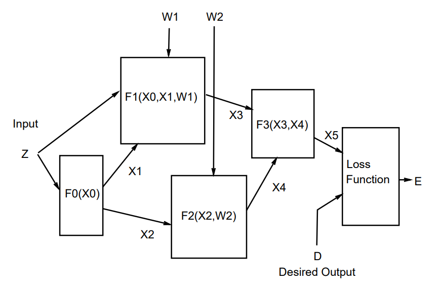
As an example, consider a system built as a cascade of modules, each of which implements a function $X_n=F_n(W_n,X_{n-1})$, where $X_n$ is a vector representing the output of the module, $W_n$ is the vector of tunable parameters in the module (a subset of $W$), and $X_{n-1}$ is the module's input vector (and the previous module's output vector). The input $X_0$ to the first module is the input pattern $Z^p$. If $\partial E^p / \partial X_n$ is know, then we can compute the following using the backward recurrence

$$\begin{align} \frac{\partial E^p}{\partial W_n} = \frac{\partial F}{\partial W}(W_n,X_{n-1})\frac{\partial E^p}{\partial X_n}\\[2ex] \frac{\partial E^p}{\partial X_{n-1}} = \frac{\partial F}{\partial X}(W_n,X_{n-1})\frac{\partial E^p}{\partial X_n} \end{align}$$

where $(\partial F / \partial W)(W_n,X_{n-1})$ is the Jacobian of $F$ with respect to $W$ evaluated at the point $(W_n,X_{n-1})$, and $(\partial F / \partial X)(W_n,X_{n-1})$ is the Jacobian of $F$ with respect to $X$. The Jacobian of a vector function is a matrix containing the partial derivatives of all the outputs with respect to all the inputs:

$$J_f(x_1, \ldots, x_n) = \begin{bmatrix} \frac{\partial f_1}{\partial x_1} & \ldots & \frac{\partial f_1}{\partial x_n}\\ \vdots & \ddots & \vdots\\ \frac{\partial f_m}{\partial x_1} & \ldots & \frac{\partial f_m}{\partial x_n}\\ \end{bmatrix}$$

We can average the gradients over the training patterns to obtain the full gradient. Traditional NN's are a special case of the above where the state information $X_n$ is represented with fixed-sized vectors, and where the modules are alternated layers of matrix multiplications and component-wise sigmoid functions. However, the state information in complex recognition system is best represented by graphs with numerical information attached to the arcs. Each module, called a graph transformer (GT), takes one or more graphs as input and produces a graph as output. Networks of such modules are called graph transformer networks (GTN's).

Convolutional neural networks for isolated character recognition

In the traditional model of pattern recognition, a hand-designed feature extractor gathers relevant information from the input and eliminates irrelevant information from the input. A trainable classifier then categorizes the resulting feature vectors into classes. A fully-connected multilayer networks can be used as classifiers. However, there are several problems: 1. Images are large, increasing the capacity of the system and therefore requires a larger training set. 2. Memory requirement to store so many weights may have hardware implementation problems. 3. There is no built-in invariance with respect to translations or local distortions of the inputs. 4. The topology of the input is entirely ignored. Pixels that are nearby are highly correlated. Local correlations allow extracting and combining local features (classified as edges, corners, etc.) before recognizing spatial or temporal objects.

Convolutional networks

Convolutional networks deliver shift, scale, and distortion invariance by 1. local receptive fields; 2. shared weights (or weight replication); 3. spatial or temporal subsampling.

With local receptive fields neurons can extract elementary visual features such as oriented edges, endpoints, corners, or speech spectrograms. These features are then combined by the subsequent layers in order to detect higher order features. Elementary feature detectors that are useful on one part of the image are likely to be useful across the entire image. Units in a layer are organized in planes within which all the units share the same set of weights. The set of outputs of the units in such a plane is called a feature map. A complete convolutional layer is composed of several feature maps with different weight vectors, so that multiple features can be extracted at each location.

Units in the first hidden layer of LeNet-5 are organized in six planes, each of which is a feature map. A unit in a feature map has 25 inputs connected to a $5 \times 5$ area in the input, called the receptive field of the unit. Each unit has 25 inputs and therefore 25 trainable coefficients plus a trainable bias. Receptive fields of neighboring units overlap. All the units in a feature map share the same set of 25 weights and the same bias, so they detect the same feature at all possible locations on the input. The other feature maps in the layer use different sets of weights and biases, thereby extracting different types of local features.

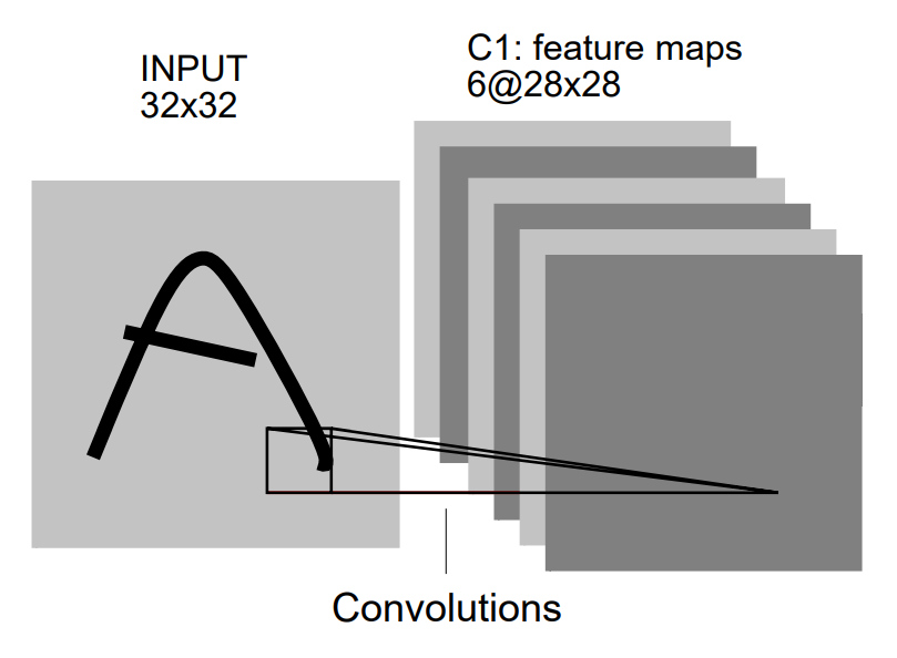
In the first hidden layer of LeNet-5, at each input location six different types of features are extracted by six units in identical locations in the six feature maps. A sequential implementation of a feature map would scan the input image with a single unit that has a local receptive field and store the states of this unit at corresponding locations in the feature map. This operation is equivalent to convolution in digital image processing, followed by an additive bias and squashing function. The kernel of the convolution is the set of connection weights used by the units in the feature map.

If the input image is shifted, the feature map output will be shifted by the same amount. This property is at the basis of the robustness of convolutional networks to shifts and distortions of the input. Once a feature has been detected, its location becomes less important. Only its approximate position relative to other features is relevant.

The precise position of each feature is not only irrelevant for identifying the pattern, it is potentially harmful, because the positions are likely to vary for different instances of the character. A simple way to reduce the precision with which the position of distinctive features are encoded in a feature map is to reduce the spatial resolution of the feature map and reducing the sensitivity of the output to shifts and distortions.

The second hidden layer in LeNet-5 is the subsampling layer. It has six feature maps, one for each feature map in the previous layer. The receptive field of each unit is a $2 \times 2$ area in the previous layer's corresponding feature map. Each unit computes the average of its four inputs, multiplies it by a trainable coefficient, adds a trainable bias, and passes the result through a sigmoid function. Contiguous units have non-overlapping contiguous receptive fields. Consequently, a subsampling layer feature map has half the number of rows and columns as the feature maps in the previous layer.

$$\begin{bmatrix} c_{11} & c_{12}\\ c_{21} & c_{22}\\ \end{bmatrix}\rightarrow \sigma(\frac{c_{11}+c_{12}+c_{21}+c_{22}}{4}k + b)$$

The trainable coefficient and bias control the effect of the sigmoid nonlinearity. If the coefficient is small, then the unit operates in a quasi-linear mode, and the subsampling layer merely blurs the input. If the coefficient is large, subsampling units can be seen as performing a "noisy OR" or a "noisy AND" function depending on the value of he bias.

A large degree of invariance to geometric transformations of the input can be achieved with progressive reduction of spatial resolution compensated by a progressive increase of the richness of the representation (the number of feature maps).

Since all the weights are learned with back propagation, convolutional networks can be seen as synthesizing their own feature extractor. The weight sharing technique has a side effect of reducing the number of free parameters, thereby reducing the capacity of the machine and reducing the gap between test error and training error. LeNet-5 has 345 308 connections, but only 60 000 trainable free parameters because of the weight sharing.

LeNet-5

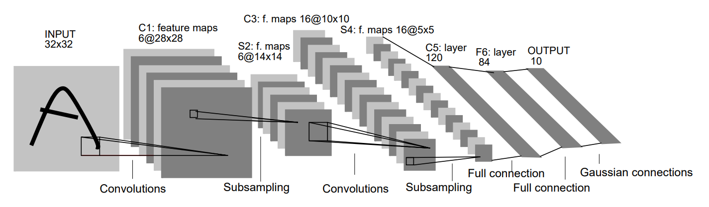
LeNet-5 has seven layers, not counting the input, all having trainable parameters. The input is $32 \times 32$ pixel image. The largest character in the database is $20 \times 20$ pixels centered in a $28 \times 28$ field. It is desirable that the potential distinctive features like endpoints appear in the center of the receptive field of the highest level feature detectors. The values of the input pixels are normalized so that the background level (white) corresponds to a value of -0.1 and the foreground (black) corresponds to 1.175, which makes the mean zero and variance one.

Convolutional layers are labeled Cx, subsampling layers are labeled Sx, and fully connected layers are labeled Fx, where x is the layer index.

Layer C1 is a convolutional layer with six feature maps, kernel size of $5 \times 5$, stride one, and output feature maps $28 \times 28$. C1 contains $(5^2 \times 1 + 1) \times 6 = 156$ trainable parameters and $(5^2 \times 1 + 1) \times 6 \times 28^2 = 122,304$ connections.

Layer S2 is a subsampling layer with six feature maps of size $14 \times 14$. Each unit is each feature map is connected to a $2 \times 2$ neighborhood in the corresponding feature map in C1. The four inputs are added, then multiplied by a trainable coefficient, and the added to a trainable bias. The result is passed through a sigmoidal function. The $2 \times 2$ receptive fields are non-overlapping. Layer S2 has $(1 + 1) \times 6 = 12$ trainable parameters and $(4 + 1) \times 14^2 \times 6 = 5,880$ connections.

Layer C3 is a convolutional layer with 16 feature maps. Each unit in each feature map is connected to several $5 \times 5$ neighborhoods at identical locations in a subset of S2's feature maps as shown below:

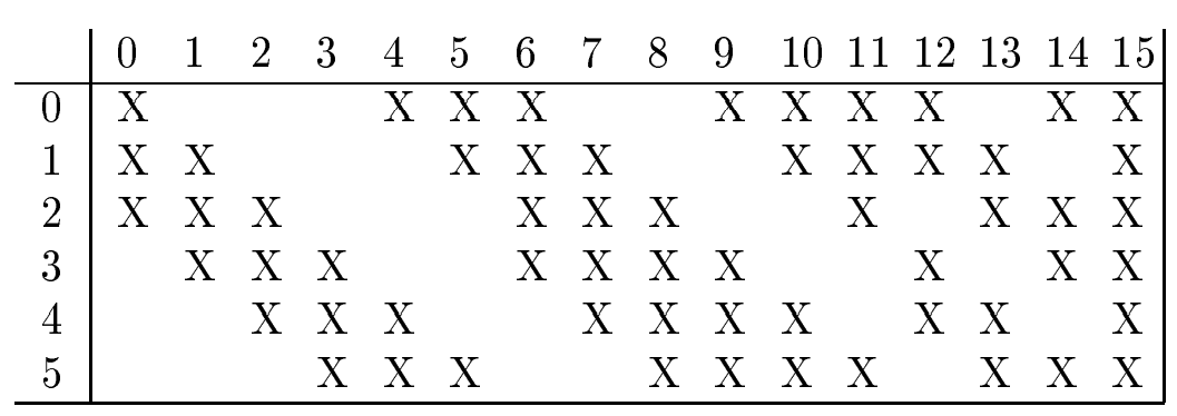
The reason to make a non-complete connection with the feature maps in the previous layer is to reduce the number of connections and break the symmetry in the network. Layer C3 has $(5^2 \times 3 + 1) \times 6 + (5^2 \times 4 + 1) \times 9 + (5^2 \times 6 + 1) = 1516$ trainable parameters and $\left[ (5^2 \times 3 + 1) \times 6 + (5^2 \times 4 + 1) \times 9 + (5^2 \times 6 + 1) \right] \times 10^2 = 151,600$ connections.

Layer S4 is a subsampling layer with 16 feature maps of size $5 \times 5$. Each unit in each feature map is connected to a $2 \times 2$ neighborhood in the corresponding feature map in C3, in a similar way as C1 and S2. Layer S4 has $(1 + 1) \times 16 = 32$ trainable parameters and $(4 + 1) \times 5^2 \times 16 = 2,000$ connections.

Layer C5 is a convolutional layer with 120 feature maps. Each unit is connected to a $5 \times 5$ neighborhood on all 16 of S4's feature maps. Layer C5 has $(5^2 \times 16 + 1) \times 120 = 48,120$ trainable parameters and $(5^2 \times 16 + 1) \times 1^2 \times 120 = 48,120$ connections. It is equivalent to a fully connected layer, but if the size of the input gets bigger, while everything else keeps the same, then the feature maps would be larger than $1 \times 1$.

Layer F6 contains 84 units and is fully connected to C5. It has $(120 + 1) \times 84 = 10,164$ trainable parameters.

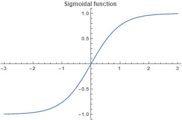
Units in layers up to F6 compute a dot product between their input vector and their weight vector, to which a bias is added. This weighted sum $a_i$ for unit $i$ is then passed through a sigmoid squashing function to produce the state $x_i$ of unit $i$

$$x_i = f(a_i)$$

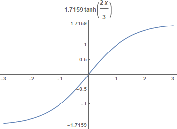
The squashing function is a scales hyperbolic tangent

$$f(a) = A \tanh (Sa)$$

where $A=1.7159$ is the amplitude of the function and $S=2/3$ determines the slope at the origin. With this choice of parameters, $f(1)=1$ and $f(-1)=-1$. Also, the second derivative $f''(a)$ is a maximum at $+1$ or $-1$, which improves the convergence.

The output layer is composed of Euclidean RBF units, one for each class with 84 inputs each. The outputs of each RBF unit $y_i$ is computes the Euclidean distance between its input vector and its parameter vector:

$$y_i = \sum_j (x_j - w_{ij})^2$$

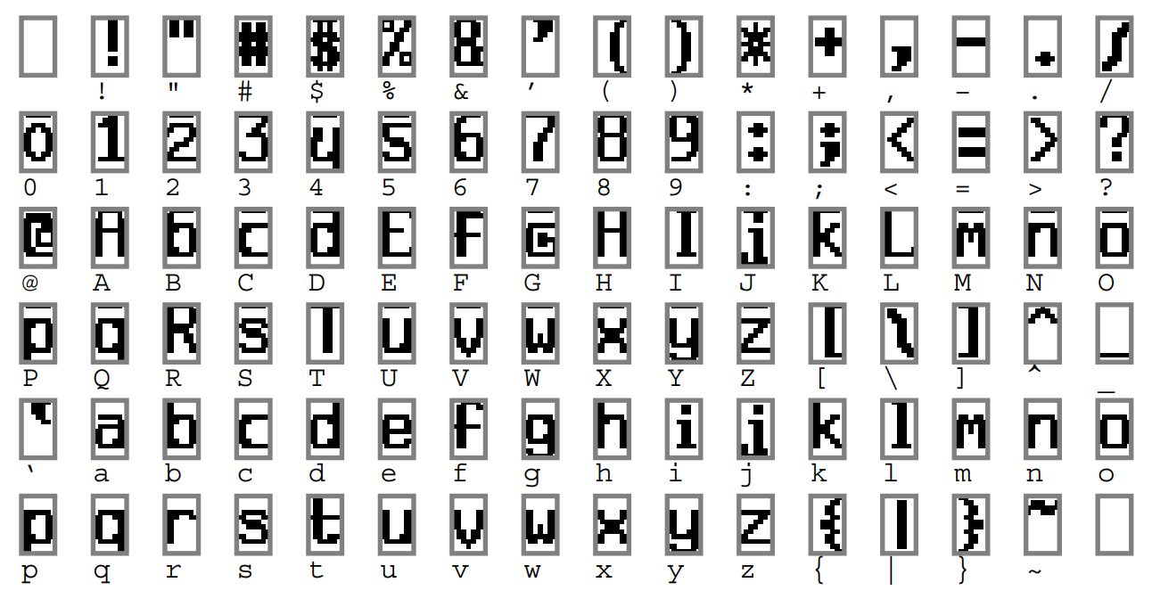
The RBF output can be interpreted as the unnormalized negative log-likelihood of a Gaussian distribution in the space of configurations of layer F6. The components of parameter vectors are chosen by hand and kept fixed initially to $-1$ or $+1$. They were designed to represent a stylized image of the corresponding character class drawn on a $7 \times 12$ bitmap. Such a representation is useful to represent printable ASCII set, because similar characters ("O", "o", and 0") will have similar output codes, so that linguistic post-processor will be able to pick the appropriate interpretation. The parameter vectors of RBF units play the role of target vectors for layer F6.

Before training, the weights are initialized with random values using a uniform distribution between $-2.4/F_i$ and $2.4F_i$, where $F_i$ is the number of inputs (fan-in) of the unit which the connection belong to. The reason for dividing by the fan-in is that the standard deviation of the weighted sums will be in the same range for each unit and fall within the normal operating region of the sigmoid.

Loss function

The loss function used in the network is the maximum likelihood estimation criterion, which is equivalent to mean squared error (MSE):

$$E(W) = \frac {1}{P} \sum_{p=1}^P y_{D^p}(Z^p,W)$$

where $y_{D^p}$ is the output of the desired output $D^p$th RBF unit, e.i. the one that corresponds to the correct class of input pattern $Z^p$. If the RBF units are allowed to adapt, the network ignores the input and sets RBF weights to zero. Therefore, the RBF units are not allowed to adapt. Also, there is no competition between the classes, so maximum a posteriori (MAP) criterion is used to pull up the penalty of the incorrect classes:

$$E(W) = \frac {1}{P} \sum_{p=1}^P \left( y_{D^p}(Z^p,W) + \log \left( e^{-j} + \sum_i e^{-y_i(Z^p,W)} \right) \right)$$

The gradient of the loss function with respect to all the weights in all the layers of the convolutional network is done with back propagation. First, partial derivatives of the loss function with respect to each connection are computed. Then the partial derivatives of all the connections that share a same parameter are added to form the derivative with respect to that parameter.

Results and comparison with other methods

The modified NIST data set

MNIST dataset is made up of two NIST data sets: SD-1 and SD-3. SD-1 was collected among high-school students, and SD-3 among Census Bureau employees. 30,000 characters written by the first 250 writers of SD-1 went to the training set, which was completed with the SD-3 examples, totaling 60,000 characters. The remaining characters of another 250 writers of SD-1 went to the test set, which was also completed with the examples from SD-3 data set. Only a subset of 10,000 images were used for the test set. Training set and test set were written by separate group of writers.

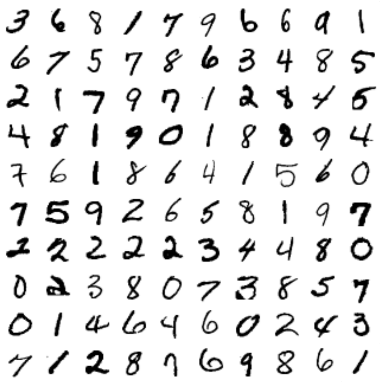
The resulting images contain grey levels as a result of anti-aliasing (image interpolation) technique used by the normalization algorithm. The images were centered in a $28 \times 28$ image by computing the center of mass of the pixels.

Results

The global learning rate was evaluated before each iteration by using the diagonal Hessian approximation on 500 samples. It was found that more training data improved the accuracy. Data augmentation was used: horizontal and vertical translations, scaling, squeezing (simultaneous horizontal compression and vertical elongation, or the reverse), and horizontal shearing. With distorted images the test error dropped to 0.8% from 0.95% without deformation. The total length of the training session was 20 passes of 60,000 patterns each.

Comparison with other classifiers

Error rates regular data / distorted images 1. Linear classifier: 12% 2. K-NN: 5.0% 3. PCA with polynomial classifier: 3.3% 4. RBF network with K-means: 3.6% 5. One-hidden-layer fully-connected NN: 4.7% / 3.6% with 300 hidden units and 4.5% / 3.8% for 1000 hidden units 6. Two-hidden-layer fully connected NN: 3.05% / 2.5% with 300-100 hidden units and 2.95% / 2.45% with 1000-150 hidden units. 7. Lenet-1: 1.7% 8. LeNet-4: 1.1% 9. Boosted LeNet-4: 0.7% on distorted images 10. Tangent distance classifier: 1.1% 11. SVM: 1.1% with poly 4, 1% with poly 5, and 0.8% with poly 9

Multi-module systems and graph transformer networks

Derivatives can be back-propagated through any arrangement of functional modules, as long as it is possible to compute Jacobians of those modules by any vector. Large and complex trainable systems need to be built out of simple, specialized modules.

A multi-module system is defined by the function implemented by each of the modules and by the graph of interconnection of the modules to each other.The graph implicitly defines a partial order according to which the modules must be updated in the forward pass. Modules may or may not have trainable parameters.

An object-oriented approach

Object-oriented programming is a convenient way to implement multi-modules system. For example, a module class can have a forward propagation and back propagation methods. The state variables of the class are assumed to contain slots for storing gradients computed during the backward pass. A sum of several variables in the forward direction is transformed into a simple fan-out (replication) in the backward direction. Conversely, a fan-out in the forward direction is transformed into a sum in the backward direction.

Special modules

NN and other techniques can be formulated in terms of modules, such as: - matrix multiplications - sigmoidal modules - convolutional layers - subsampling layers - RBF layers - softmax layers - loss functions

Commonly used modules can have backpropagation methods. In general, the backpropagation method of a function $F$ is a multiplication by the Jacobian of $F$.

Certain non-differentiable modules can be inserted in a multimodule system without adverse effects, such as: - multiplexer module - minimum module

These ideas were implemented in the software called SN3.1, which was a predecessor of Pytorch.

GTN's

The previous description assumed that each module has a fixed-sized vector of weights, inputs, and outputs, which has limited flexibility in speech recognition and handwriting recognition applications. Directed graphs can encode probability distributions over sequences of vectors or symbols. Stochastic grammars is a special case of directed graphs in which the vectors contain probabilities and symbolic information.

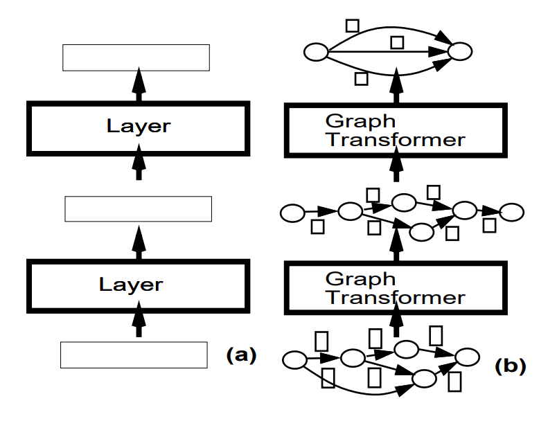
Viewing the system as a network of modules that take one or several graphs as input and produce graphs as output is convenient for building a complex system. Modules in a GTN communicate their states and gradients in the form of directed graphs whose arc carry numerical information (scalars or vectors). States in GTN are represented as graphs.

Gradient-based learning procedures are not limited to networks of simple modules that communicate through fixed-size vectors but can be generalized to GTN's, as long as differentiable functions are used to produce the numerical data in the output graph from the numerical data in the input graph and the functions parameters.

Multiple object recognition: HOS

Most recognizers can only deal with one character at a time, therefore for recognizing strings of characters it is required to segment the string into individual character images. Training a recognizer by optimizing a global criterion is better than training it on presegmented characters, because the recognizer can learn to reject missegmented characters.

Segmentation graph

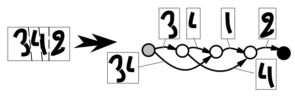
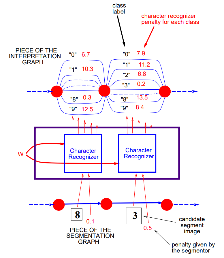
Heuristic oversegmentation avoids making hard decision about the segmentation by taking a large number of different segmentations into consideration. Good candidate locations for cuts can be found by locating minima in the vertical projection profile, or minima of the distance between the upper and lower contours of the word. By generating more cuts than necessary, there is a higher probability that the correct set of cuts will be included. Alternative segmentations are represented by a segmentation graph. Each internal node is associated with a candidate cut. Each arc between a source node and a destination node is associated with an image that contains all the ink between the cuts. Each individual piece of ink is associated with an arc.

Recognition transformer and Viterbi transformer

A simple GTN to recognize character strings is composed of two GT's called the recognition transformer $T_{\text{rec}}$ and the Viterbi transformer $T_{\text{vit}}$. The goal of the recognition transformer is to generate an interpretation graph $G_{\text{int}}$, that contains all possible interpretations for all the possible segmentations of the input. Each path in $G_{\text{int}}$ represents one possible interpretation of one particular segmentation of the input. Viterbi transformer extracts the best interpretation from $G_{\text{int}}$.

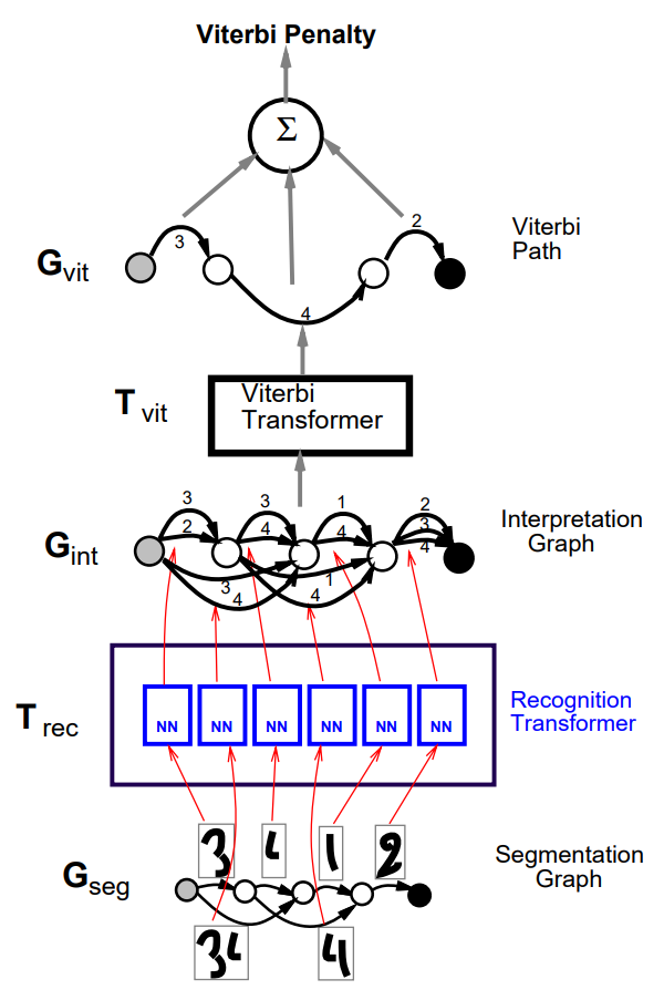
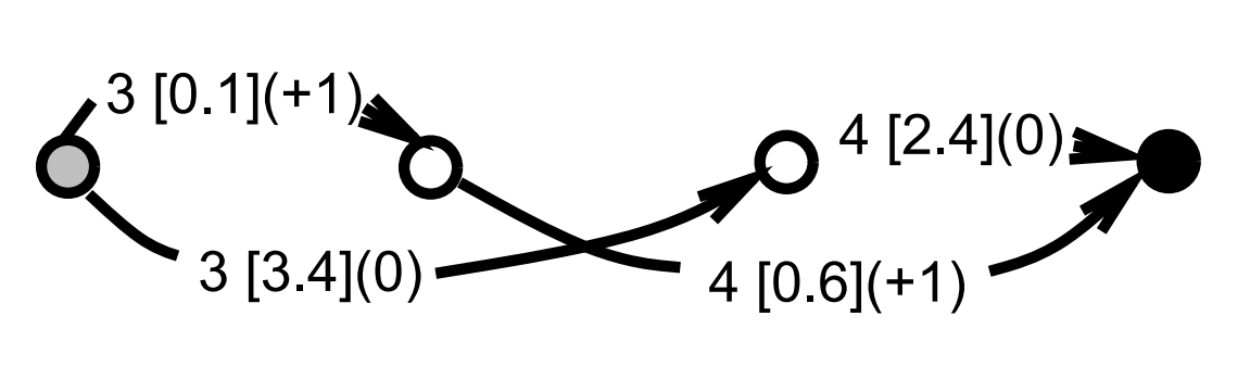
The recognition transformer $T_{\text{rec}}$ applies recognizer for single characters to the images on the arcs of the segmentation graph $G_{\text{seg}}$. In the resulting set of arcs, there is one arc for each possible class with combined penalty (segmenter and recognizer) of the image associated with the corresponding arc in $G_{\text{seg}}$. The penalty of a particular interpretation for a particular segmentation is given by the sum of the arc penalties along the corresponding path in the interpretation graph.

The Viterbi transformer produces a graph $G_{\text{vit}}$ with a single path, which is of least cumulated penalty in the interpretation graph $G_{\text{int}}$. The Viterbi transformer uses Viterbi algorithm to find the shortest path in a graph efficiently (explanation video). Let $c_i$ be the penalty associated to arc $i$, with source node $s_i$, destination node $d_i$, and a label $l_i$. Each node $n$ is associated with a cumulated Viterbi penalty $v_n$. The start node is initialized with the cumulated penalty $v_\text{start}=0$. The other nodes cumulated penalties $v_n$ are computed recursively from the $v$ values of their parent nodes, through the upstream arcs $U_n=\{$ arc $i$ with destination $d_i=n\}$

$$v_n = \min_{i \in U_n} (c_i + v_{s_i})$$

The value of $i$ for each node $n$ which minimizes the right-hand side is denoted $m_n$, the minimizing entering arc. When the end node $v_\text{end}$ is reached, the total penalty of the path with the smallest total penalty is obtained. To obtain the Viterbi path with nodes $n_1 \ldots n_T$ and arcs $i_1 \ldots i_{T-1}$, we trace back these nodes and arcs, starting from the end node, and recursively using the minimizing entering arc until the start node is reached. The label sequence is then read off the arcs of the Viterbi path.

Global training for graph transformer networks

The recognizer is assumed to be pre-trained. There are several architectures that use gradient-based methods for training GTN-based handwriting recognizers at the string level.

Viterbi training

Viterbi algorithm selects the path in the interpretation graph with the lowest penalty, which ideally should be associated with the correct label sequence as often as possible. The obvious loss function to minimize is the average over the training set of the penalty of the path associated with the correct label sequence that has the lowest penalty. The gradient of this loss function can be computed by back propagation through the GTN architecture.

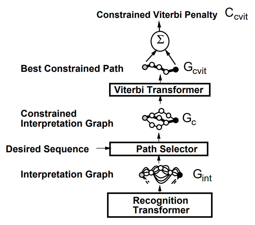
There is an extra GT called path selector inserted between the interpretation graph and the Viterbi transformer. This transformer takes the interpretation graph and the desired label sequence and extracts those paths that contain the correct (desired) label sequence, called the constrained interpretation graph $G_c$. The constrained interpretation graph is then sent to the Viterbi transformer which produces a graph $G_{\text{cvit}}$ with a single path. Finally, a path scorer transformer takes $G_{\text{cvit}}$ and computes its cumulated penalty $C_{\text{cvit}}$ by adding up the penalties along the path. The output of this GTN is the loss function for the current pattern

$$E_{\text{vit}} = C_{\text{cvit}}$$

The label must contain the sequence of desired character labels. The gradients are back propagated from the loss function $E_{\text{vit}}$ down to the preceding modules. The partial derivatives of the loss function $E_{\text{vit}}$ with respect to the individual penalties on the constrained Viterbi path $G_{\text{cvit}}$ are equal to one, since the loss is simply the sum of those penalties. The partial derivatives of $E_{\text{vit}}$ with respect to the penalties on the arcs of the constrained graph $G_c$ are one for those arcs that appear in the constrained Viterbi path $G_{\text{cvit}}$ and zero for those that do not. The Viterbi transformer is nothing more than a collection of $\min$ functions and adders put together. Back propagation through the path selector transformer is similar: arcs in $G_{\text{int}}$ that appear in $G_v$ have the same gradient as the corresponding arc in $G_c$, and the other arcs have a gradient of zero.

During the forward propagation through the recognition transformer, one instance of the recognizer for single character was created for each arc in the segmentation graph. Since each arc penalty in $G_{\text{int}}$ was produced by an individual output of a recognizer instance, we have a gradient (one or zero) for each output of each instance of the recognizer. Recognizer outputs that have a nonzero gradient are part of the correct answer and will therefore have their value pushed down.

For each recognizer instance, we obtain a vector of partial derivatives of the loss function with respect to the recognizer instance parameters. All the recognizer instances share the same parameter vector, since they are merely clones of each other, therefore the full gradient of the loss function with respect to the recognizer's parameter vector is simply the sum of the gradient vectors produced by each recognizer instance.

The training architecture has some flaws: 1. If the recognizer is a simple NN with sigmoid output units, the minimum is attained when it ignores the input and set its output to a constant vector with small values for all the components. It is called the collapse problem. 2. If the recognizer's output layer contains RBF units with fixed parameters, the collapse does not occur, however the loss function has a "flat spot" for a trivial solution with constant recognizer output. It is a saddle point. 3. If the parameters of the RBF units are allowed to adapt, the collapse problem reappears again.

Discriminative Viterbi training

A modification of the training criterion can circumvent the collapse problem and produce more reliable confidence values. The idea is to not only minimize the cumulated penalty of the lowest penalty path with correct interpretation, but also to increase the penalty of competing and possibly incorrect paths that have a dangerously low penalty. This type of criterion is called discriminative because it plays the good answers against the bad ones.

The discriminative criterion is the difference between the penalty of the best correct path and the penalty of the best path (correct and incorrect). The loss function reduces the risk of collapse because it forces the recognizer to increase the penalty of wrongly recognized objects. It can be seen as error correction procedure to minimize the difference between the desired output on the left half to the actual output on the right half.

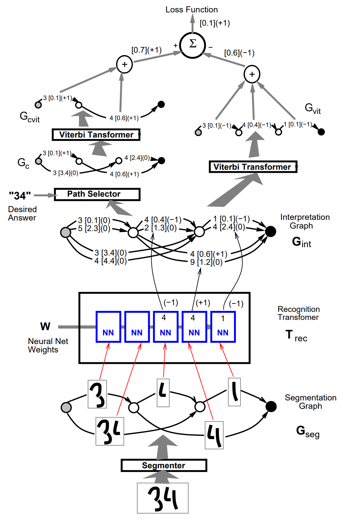
Let the discriminative Viterbi loss function be denoted $E_{\text{dvit}}$, and let us call $C_{\text{cvit}}$ the penalty of the Viterbi path in the constained graph and $C_{\text{vit}}$ the penalty of the Viterbi path in the unconstrained interpretation graph

$$E_{\text{dvit}} = C_{\text{cvit}} - C_{\text{vit}}$$

$E_{\text{vit}}$ is non-negative since the constrained graph is a subset of the paths in the interpretation graph, and the Viterbi algorithm selects the path with the lowest total penalty. In the ideal case, two paths $C_{\text{cvit}}$ and $C_{\text{vit}}$ coincide, and $E_{\text{dvit}}$ is zero.

Back propagation of the gradients in the left half is the same as in the nondiscriminative Viterbi training. The gradients back propagated through the right half of the GTN are multiplied by $-1$, since $C_{\text{vit}}$ contributes to the loss with a negative sign. The gradients contributions from the right half and the left half must be added, because the penalties on $G_{\text{int}}$ arcs are sent to the two halves through a "Y" connection in the forward pass.

Arcs in $G_{\text{int}}$ that appear neither in $G_{\text{vit}}$ nor in $G_{\text{cvit}}$ have a gradient of zero. Arcs that appear in both $G_{\text{vit}}$ and $G_{\text{cvit}}$ also have a gradient of zero. If an arc appears in $G_{\text{cvit}}$ but not in $G_{\text{vit}}$, the gradient is $+1$. The arc should have had a lower penalty to make it to $G_{\text{vit}}$. If an arc is in $G_{\text{vit}}$ but not in $G_{\text{cvit}}$, the gradient is $-1$. The arc had a low penalty, but it should have had a higher penalty since it is not part of the desired answer.

The main problem is that the criterion does not build a margin between the classes. The gradient is zero as soon as the penalty of the constrained Viterbi path is equal to that of the Viterbi path. It would be desirable to push up the penalties of the wrong paths when they are dangerously close to the good one.

Forward scoring and forward training

Imagine the lowest penalty paths corresponding to several different segmentation produced the same answer (the same label sequence). Then the overall penalty for the interpretation should be smaller than the penalty obtained when only one path produced that interpretation, because multiple paths with identical label sequences are more evidence that the label sequence is correct. Using the probabilistic interpretation, the penalties can be viewed as negative log posteriors, which should be the sum of posteriors for all the paths that produce that interpretation, i.e. the negative logarithm of the sum of the negative exponentials of the penalties of the individual paths.

Forward algorithm computes the penalty for a particular interpretation, which is called the forward penalty. Running the forward algorithm on the corresponding constrained graph for a given interpretation produces the forward penalty for that interpretation. The forward algorithm is similar to Viterbi algorithm. The incoming cumulated penalties at each node are computed the following way:

$$f_n = \text{logadd} {i \in U_n} (c_i + f{s_i})$$

where $f_\text{start} = 0$, $U_n$ is the set of upstream arcs of node $n$, $c_i$ is the penalty on arc $i$, and

$$\text{logadd}(x_1, x_2, \ldots, x_n) = -\log \left( \sum_{i=1}^n e^{-x_i} \right)$$

Note that because of numerical inaccuracies, it is better to factorize the largest $e^{-x_i}$ (corresponding to the smallest penalty) out of the logarithm. The forward penalty is always lower than the cumulated penalty on any of the paths, but if one path "dominates" (with a much lower penalty), its penalty is almost equal to the forward penalty.

Viterbi transformers are replaced with forward scorers. Interpretation graph is taken as input to produce the forward penalty on output. The penalties of all the paths that contain the correct answer are lowered, instead of just that of the best one.

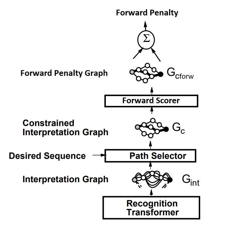
Computing derivatives for forward penalties are different from the Viterbi transformer, because all the arcs in the constrained interpretation graph $G_c$ have an influence on the loss function $E_{\text{forw}}$, but arcs that belong to low-penalty paths have a stronger influence. Computing derivatives of the loss function $E_{\text{forw}}$ with respect to the forward penalties $f_n$ at each node $n$ of a graph is done by back propagation through the graph $G_c$

$$\frac{\partial E_{\text{forw}}}{\partial f_n} = e^{-f_n} \sum_{i \in D_n} \frac{\partial E_{\text{forw}}}{\partial f_{d_i}} e^{f_{d_i}-c_i}$$

where $D_n = \{$ arc $i$ with source $d_i=n \}$ is the set of downstream arcs from node $n$. The derivatives with respect to the arc penalties are computed as following:

$$\frac{\partial E_{\text{forw}}}{\partial c_i} = \frac{\partial E_{\text{forw}}}{\partial f_{d_i}} e^{-c_i-f_{s_i}+f_{d_i}}$$

Back propagation through the path selector is the same as before. The derivative with respect to $G_{\text{int}}$ arcs that have an alter ego in $G_c$ are simply copied from the corresponding arc in $G_c$. The derivatives with respect to the other arcs are zero.

Discriminative forward training

The criterion corresponds to maximization of the posterior probability of choosing the paths associated with the correct interpretation:

$$P_\text{post} = \frac{e^{-C_{\text{cforw}}}}{e^{-C_{\text{forw}}}}$$

Note that the forward penalty of the constrained graph is always larger or equal (ideally) to the forward penalty of the unconstrained interpretation graph. Let the discriminative forward loss $E_\text{dforw}$ be the difference of the forward penalty of the constrained graph $C_\text{cforw}$ and the forward penalty of the complete interpretation graph $C_\text{forw}$:

$$E_\text{dforw} = C_\text{cforw} - C_\text{forw}$$

$E_\text{dforw}$ is always positive since the constrained graph is a subset of the paths in the interpretation graph, and the forward penalty of a graph is always smaller than the forward penalty of a subgraph of this graph. Ideally, the penalties of incorrect paths are infinitely large, so the two forward penalties coincide and $E_\text{dforw}$ is zero.

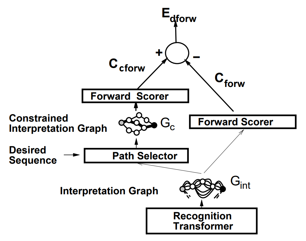
Derivatives are back propagated through the left half of the GTN down to the interpretation graph. Derivatives are negated and back propagated through the right-half, and the result for each arc is added to the contribution from the left half. Therefore, each arc in $G_\text{int}$ has a derivative.

The derivative is very large if an incorrect path has a lower penalty than all the correct paths. The derivatives with respect to arcs that are part of low-penalty incorrect path have a large negative derivative. If the penalty of a path associated with the correct interpretation is much smaller than all other paths, the loss function is close to zero and almost no gradient is back propagated.

Conclusions

• It has been shown that the application of gradient-based learning to CNN allows learning appropriate features from examples
• Instead of taking hard segmentation decision too early, use HOS to generate and evaluate a large number of hypotheses in parallel
• Training multimodule systems to optimize a global measure of performance does not require time consuming hand-truthing and yields better performance because the modules cooperate toward a common goal
• Proposed a unified framework in which generalized transduction methods are applied to graphs representing a weighted set of hypotheses about the input
• The promising SDNN approach avoids explicit segmentation altogether; simultaneous automatic learning of segmentation and recognition can be achieved with gradient-based learning methods