Gradient descent

Learning data

We will use MNIST data set to learn to recognize digits. MNIST is a modified subset of two data sets collected by the National Institute of Standards and Technology. It has 60,000 images to be used as training data and 10,000 images to be used as test data. The training images and test images are drawn by separate groups of people.

For convenience we will regard each training input $x$ as a $28 \times 28 = 784$-dimensional vector. Each entry in the vector represents the gray value for a single pixel in the image. We will denote the corresponding desired output (also called label) by $y = y(x)$ where $y$ is a 10-dimensional vector. For example, if a particular training image $x$ depicts a 6, then $y(x) = (0, 0, 0, 0, 0, 0, 1, 0, 0, 0)^T$ is the desired output from the network. Note that $T$ here is the transpose operation, turning a row vector into an ordinary (column) vector.

Matrix-based notation

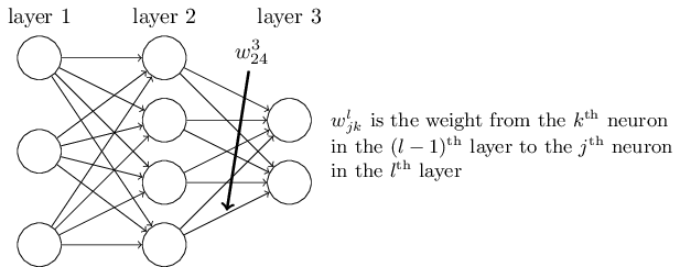
We will use $w^l_{jk}$ to denote the weight for the connection from the $k^{\text{th}}$ neuron in the $(l-1)^{\text{th}}$ layer to the $j^{\text{th}}$ neuron in the $l^{\text{th}}$ layer. So, for example, the diagram below shows the weight on a connection from the fourth neuron in the second layer to the second neuron in the third layer of a network:

For example, the weights matrix in layer 3 may look like the following:

     k=1     k=2      k=3     k=4
[[ 0.3490, 0.2552,  1.7718, -0.6382 ],  j=1
 [ 1.5340, 0.2998, -1.0761, -1.4656 ]]  j=2

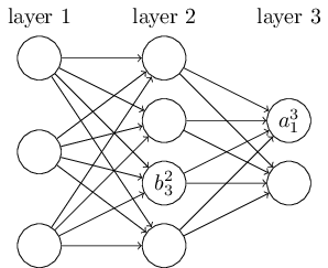
Similarly, we will use $b_j^l$ for the bias of the $j^{\text{th}}$ neuron in the $l^{\text{th}}$ layer and $a_j^l$ for the activation of the $j^{\text{th}}$ neuron in the $l^{\text{th}}$ layer.

The bias and activation matrices have only one column. Therefore, we can also call them vectors. For example, a bias matrix in layer 2 may look like this:

[[-1.2871],  j=1
 [-1.7834],  j=2
 [ 0.6244],  j=3
 [ 0.6702]]  j=4

The activation $a_j^l$ of the $j^{\text{th}}$ neuron in the $l^{\text{th}}$ layer is related to the activation in the $(l-1)^{\text{th}}$ layer by the equation

$$ \begin{align} a_j^l = \sigma \left( \sum_k w_{jk}^l a_k^{l-1}+ b_j^l \right), \tag{6} \end{align} $$

where the sum is over all neurons $k$ in the $(l-1)^{\text{th}}$ layer. Now we define a weight matrix $w^l$, bias vector $b^l$ and activation vector $a^l$ for each layer $l$. With this notation we can simplify the Equation (6) in the vectorized form:

$$ \begin{align} a^{l} = \sigma(w^l a^{l-1}+b^l). \tag{7} \end{align} $$

where we apply sigmoid function $\sigma$ to every element in the resulting vector. Note that the notation simplifies the computation because we can multiply two matrices without transposing any one of them.

We call $z^l$ the weighted input to the neurons in layer $l$. It is the intermediate quantity used to compute the activation vector $a^l$:

$$ \begin{align} z^l \equiv w^l a^{l-1}+b^l. \tag{8} \end{align} $$

It is worth noting that $z^l$ has components $z_j^l = \sum_k w_{jk}^l a_k^{l-1}+ b_j^l$, that is $z_j^l$ is just the weighted input to the activation function for neuron $j$ in layer $l$. Also, the activation function could be different for each layer. Specifically, in many implementations the activation function for the output layer is different from the activation function in the hidden layers.

Cost function

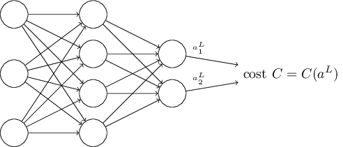
The objective of learning is to find an algorithm which lets us find weights and biases so that the output from the network $a(x)$ approximates the desired output $y(x)$ for all training inputs $x$. To quantify how well we are achieving this goal we define a cost function (which is sometimes referred to as a loss, objective, or empirical risk function):

$$ \begin{align} C(w,b) \equiv \frac{1}{2n} \sum_x \| y(x) - a^L(w,b)\|^2, \tag{9} \end{align} $$

where $n$ is the total number of training examples; the sum is over all individual training examples $x$; $y = y(x)$ is the corresponding desired output; $L$ denotes the number of layers in the network; and $a^L = a^L(w,b)$ is the vector of activations output from the network when $x$ is input. The output $a$ depends on all matrices $w$ and $b$ for each layer as well as on the input $x$ (the dependence on $x$ is not indicated explicitly here). The notation $\| v \|$ denotes the magnitude or the Euclidean norm of vector $v$. We add an extra factor of $\frac12$ in order to simplify the derivative for the gradient.

We will call $C$ the quadratic cost function, which is also called the mean squared error (MSE). We will explore other cost functions later, but there is a justification for using squared error function as a default choice.

The quadratic cost function $C$ is non-negative and $\approx 0$ when the output $a^L(w,b)$ for all training inputs $x$ is approximately equal to the desired output $y(x)$, in which case we say that the training algorithm has done a good job. By contrast, it is not doing so well when $C$ is large. Therefore, the aim of a training algorithm is to minimize the cost $C$ as a function of all weights and biases in the network. We will do that using an algorithm known as the gradient descent.

But first we need to make two assumptions about our cost function:

1. The cost function can be written as an average $C = \frac{1}{n} \sum_x C_x$ over cost functions $C_x$ for individual training examples $x$. This is true for the quadratic cost function, where the cost for a single training example is $C_x = \frac{1}{2} \|y-a^L \|^2$. We need this assumption because backpropagation lets us compute the partial derivatives $\frac{\partial C_x}{\partial w}$ and $\frac{\partial C_x}{\partial b}$ for a single training example. Then we compute $\frac{\partial C}{\partial w}$ and $\frac{\partial C}{\partial b}$ by averaging over individual training examples.

2. The cost can be written as a function of the outputs from the neural network. The quadratic cost function satisfies this requirement, because the quadratic cost for a single training example $x$ may be written as a function of the output activations:

$$ \begin{align} C_x = \frac{1}{2} \|y-a^L\|^2 = \frac{1}{2} \sum_j (y_j-a_j^L)^2. \tag{10} \end{align} $$

Note that the input training example $x$ is fixed, and so the desired output $y$ is also a fixed parameter. Therefore, we regard cost $C_x$ as a function of output activations $a^L$ alone, with $y$ as being merely a parameter that helps to define the cost function. This observation helps us simplify calculation of gradient by appliying the chain rule.

Gradient descent

We minimize quadratic cost instead of maximizing the number of correctly classified images by the network because quadratic cost is a differentiable function which will allow us to improve the performance by adjusting weights and biases. In contrast, changing weights and biases may not immediately change the number of correctly classified images. This is why we focus first on minimizing the quadratic cost, and only after that we will examine the classification accuracy.

Suppose we are trying to minimize some function $C$. This could be any real-valued function of two variables $C = C(v_1, v_2)$. If we move by a small amount $\Delta v_1$ in the $v_1$ direction, and by a small amount $\Delta v_2$ in $v_2$ direction, we can use multivariable calculus linear approximation to approximate the change in $C$ as the following:

$$ \begin{align} \Delta C \approx \frac{\partial C}{\partial v_1} \Delta v_1 + \frac{\partial C}{\partial v_2} \Delta v_2. \tag{11} \end{align} $$

In order to minimize function $C$, we are going to find a way of choosing $\Delta v_1$ and $\Delta v_2$ to make $\Delta C$ negative. We will define $\Delta v$ to be the vector of changes in $v$, $\Delta v \equiv (\Delta v_1, \Delta v_2)^T$, where $T$ is the transpose operation. We will define the gradient vector of $C$ as the following:

$$ \begin{align} \nabla C \equiv \left( \frac{\partial C}{\partial v_1}, \frac{\partial C}{\partial v_2} \right)^T. \tag{12} \end{align} $$

With these definitions, we can rewrite the Expression (11) for $\Delta C$ as the dot product of two vectors:

$$ \begin{align} \Delta C \approx \nabla C \cdot \Delta v, \tag{13} \end{align} $$

or in matrix notation

$$ \begin{align} \Delta C \approx \nabla C^T \Delta v. \tag{13.1} \end{align} $$

This equation relates changes in $v$ to changes in $C$, and lets us see how to choose $\Delta v$ so as to make $\Delta C$ negative. In particular, we choose

$$ \begin{align} \Delta v = -\eta \nabla C, \tag{14} \end{align} $$

where $\eta$ is a small, positive parameter (known as the learning rate). Geometrically, we choose the vector $\Delta v$ to be in the opposite direction to $\nabla C$, modified by the learning rate $\eta$.

Equation (13) tells us that $\Delta C \approx \nabla C \cdot (-\eta \nabla C) = -\eta \|\nabla C\|^2$. Because the square of the magnitude of the gradient $\|\nabla C\|^2 \geq 0$, this guarantees that $\Delta C \leq 0$, i.e., $C$ will always decrease, never increase, if we change $v$ according to the prescription in (14).

We will use Equation (14) for our gradient descent algorithm to compute a value for $\Delta v$, then move the position of $v$ by that amount:

$$ \begin{align} v \rightarrow v' = v + \Delta v = v -\eta \nabla C. \tag{15} \end{align} $$

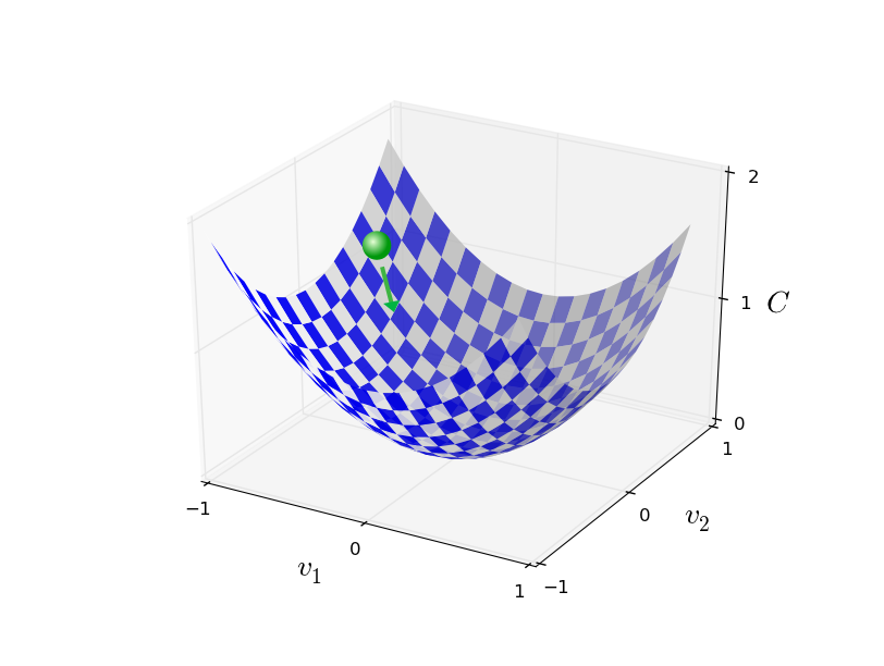
Then we will use this update rule again to make another move. If we keep doing this, over and over, we will keep decreasing $C$ to a point of global minimum. We can visualize the gradient descent in the following picture:

To make gradient descent work correctly, we need to choose the learning rate $\eta$ to be small enough that Equation (13) is a good approximation. Otherwise we might end up with $\Delta C \gt 0$. Also, we don't want $\eta$ to be too small, since that will make the changes $\Delta v$ tiny, and thus the gradient descent algorithm will work very slowly. In practice, $\eta$ is often varied so that Equation (13) remains a good approximation, but the algorithm isn't too slow.

The gradient descent algorithm also works when $C$ is a function of many variables. Suppose that $C$ is a function of $m$ variables, $v_1,\ldots,v_m$. Then the change $\Delta C$ in $C$ produced by a small change $\Delta v = (\Delta v_1, \ldots, \Delta v_m)^T$ is

$$ \begin{align} \Delta C \approx \nabla C \cdot \Delta v, \tag{16} \end{align} $$

where the gradient $\nabla C$ is the vector

$$ \begin{align} \nabla C \equiv \left(\frac{\partial C}{\partial v_1}, \ldots, \frac{\partial C}{\partial v_m}\right)^T. \tag{17} \end{align} $$

Just as for the two variable case, we can choose

$$ \begin{align} \Delta v = -\eta \nabla C, \tag{18} \end{align} $$

and we are guaranteed that our (approximate) Expression (16) for $\Delta C$ will be negative. This gives us a way of following the gradient to a minimum, even when $C$ is a function of many variables, by repeatedly applying the update rule

$$ \begin{align} v \rightarrow v' = v-\eta \nabla C. \tag{19} \end{align} $$

Now we can use gradient descent to find weights $w_k$ and biases $b_l$ which minimize the cost in equation (10). We will restate the gradient descent update rule, with the weights and biases replacing the variables $v_j$:

$$ \begin{align} w_k \rightarrow w_k' & = w_k-\eta \frac{\partial C}{\partial w_k} \tag{20}\\[2ex] b_l \rightarrow b_l' & = b_l-\eta \frac{\partial C}{\partial b_l}. \tag{21} \end{align} $$

By repeatedly applying this update rule we can find a minimum of the cost function. In other words, this is a rule which can be used to learn in a neural network.

Notice that we compute the gradients $\nabla C_x$ for each training input, $x$, and then averaging them, so $\nabla C = \frac{1}{n} \sum_x \nabla C_x$. Sometimes we might want to sum over the cost of individual examples instead of averaging them. This approach is useful when we don't know the total number of training examples. Also, we can omit $\frac{1}{m}$ term in mini-batch update rule (where $m$ is the number of training examples in one mini-batch, see more below). This is equivalent to rescaling the learning rate $\eta$. Unfortunately, when the number of training inputs is very large, summing over all the gradients can take a long time, leading to slow learning.

Stockastic gradient descent

A method called stochastic gradient descent can be used to speed up learning. The idea is to estimate the gradient $\nabla C$ by computing $\nabla C_x$ for a small sample of randomly chosen training inputs. By averaging over this small sample it turns out that we can quickly get a good estimate of the true gradient $\nabla C$, and this helps speed up gradient descent, and thus learning. It works like political polling: it is easier to carry out a poll than running a full election.

To implement stochastic gradient descent, we choose a small number $m$ of randomly chosen training inputs. We label those random training inputs $X_1, X_2, \ldots, X_m$, and refer to them as a mini-batch. Provided the sample size $m$ is large enough we expect that the average value of the $\nabla C_{X_j}$ sill be roughly equal to the average over all $\nabla C_x$, that is

$$ \begin{align} \frac{\sum_{j=1}^m \nabla C_{X_{j}}}{m} \approx \frac{\sum_x \nabla C_x}{n} = \nabla C, \tag{22} \end{align} $$

where the second sum is over the entire set of training data. By swapping sides we get

$$ \begin{align} \nabla C \approx \frac{1}{m} \sum_{j=1}^m \nabla C_{X_{j}}, \tag{23} \end{align} $$

confirming that we can estimate the overall gradient by computing gradients just for the randomly chosen mini-batch. Then stochastic gradient descent update rule will be

$$ \begin{align} w_k \rightarrow w_k' & = w_k-\frac{\eta}{m} \sum_j \frac{\partial C_{X_j}}{\partial w_k} \tag{24}\\ b_l \rightarrow b_l' & = b_l-\frac{\eta}{m} \sum_j \frac{\partial C_{X_j}}{\partial b_l}, \tag{25} \end{align} $$

where the sums are over all the training examples $X_j$ in the current mini-batch. Then we pick out another randomly chosen mini-batch and train with those. And so on, until we've exhausted all of the training inputs, which is said to complete an epoch of training. At that point we start over with a new training epoch.

Sometimes it helps to visualize higher dimensions to understand how gradient descent works. We can learn techniques for representing higher dimensions on this forum.

Geometric intuition of the gradient descent

We want to minimize the cost function $\Delta C \approx \nabla C \cdot \Delta v$ (Equation 13) by finding the value of $\Delta v$ that does the trick. The geometric interpretation of the gradient says that the gradient $\nabla C$ is the vector of the steepest ascent from a given point. If we divide the gradient vector $\nabla C$ by its magnitude $\| \nabla C \|$, we get a unit vector in the direction of the steepest ascent. Multiplying this unit vector by $-1$ gives us a unit vector in the opposite direction of the steepest ascent. Finally, we choose a fixed step size to be a scalar $\epsilon \gt 0$, which we multiply by the unit vector in the opposite direction of steepest ascent and will obtain a move $\Delta v$ in the direction of steepest descent:

$$ \begin{align} \Delta v = -\epsilon \frac {\nabla C} {\| \nabla C \|} = -\eta \nabla C \tag{26} \end{align} $$

Note that $\eta = \frac {\epsilon} {\| \nabla C \|}$ is a positive scalar value known as the learning rate.

Finally, we observe that the change in the cost function will always be negative because the learning rate and the square magnitude of the gradient vector are always positive:

$$ \begin{align} \Delta C \approx \nabla C \cdot (-\eta \nabla C) = -\eta \|\nabla C\|^2 \lt 0 \tag{27} \end{align} $$

which can be expressed equally well in matrix notation as

$$ \begin{align} \Delta C \approx \nabla C^T (-\eta \nabla C) = -\eta \|\nabla C\|^2 \lt 0 \tag{27.1} \end{align} $$

Proof by using Schwarz inequality

After getting a geometric intuition about the gradient descent algorithm, we are going to prove that gradient descent is the optimal strategy for searching for a minimum of the cost function $C$. We want to minimize the cost function $\Delta C \approx \nabla C \cdot \Delta v$ (Equation 13) by finding the value of $\Delta v$ that does the trick. Let us choose $\epsilon = \|\Delta v\| \in \mathbb{R} \gt 0$ to be our step size. By Cauchy-Schwarz inequality we know that

$$ \begin{align} |\nabla C \cdot \Delta v| \le \|\nabla C\| \|\Delta v\|. \tag{28} \end{align} $$

Recall that

$$ \begin{align} |x| \le a \iff x \in [-a,a]. \tag{29} \end{align} $$

Therefore,

$$ \begin{align} \min(\nabla C \cdot \Delta v) = -\|\nabla C\| \|\Delta v\|. \tag{30} \end{align} $$

We need to find $\Delta v$ such that

$$ \begin{align} \nabla C \cdot \Delta v = -\|\nabla C\| \|\Delta v\| = -\epsilon \|\nabla C\|. \tag{31} \end{align} $$

Since

$$ \begin{align} \nabla C \cdot \nabla C = \|\nabla C\|^2, \tag{32} \end{align} $$

we conclude the following:

$$ \begin{align} \frac{\nabla C \cdot \nabla C} {\|\nabla C\|} & = \|\nabla C\| \\[2ex] -\epsilon \frac{\nabla C \cdot \nabla C} {\|\nabla C\|} & = -\epsilon \|\nabla C\| \\[2ex] -\epsilon \frac{\nabla C \cdot \nabla C} {\|\nabla C\|} & = \nabla C \cdot \Delta v, \\[2ex] \Delta v = -\epsilon \frac{\nabla C} {\|\nabla C\|} & = -\eta \nabla C \quad \blacksquare \tag{33} \end{align} $$

Adapted from Michael A. Nielsen, "Neural Networks and Deep Learning"