Deep learning

Learning problem with deep neural networks

Convolutional neural networks

Previously we used neural network with fully connected layers where every neuron in the network is connected to every neuron in adjacent layers:

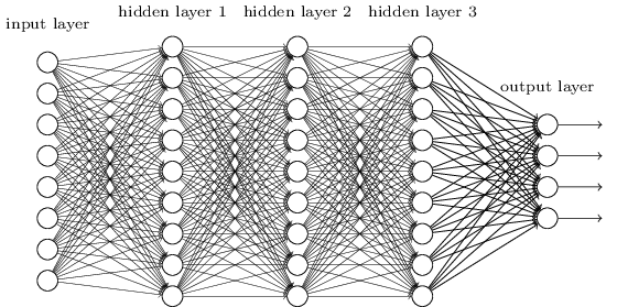
However, for image classification it is strange to use networks with fully connected layers because such a network does not account for spatial structure of the images: it treats input pixels which are far apart and close together the same. In contrast, convolutional neural networks use a special architecture that works exceptionally well for classifying images. Convolutional neural networks use three basic ideas: local receptive fields, shared weights, and pooling.

Local receptive fields

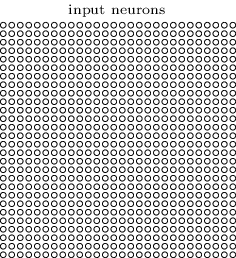
In the fully-connected layers we represented the image as a vertical stack of neurons. In a convolutional network, we will think of the inputs as $28 \times 28$ square of neurons:

This time we won't connect every input pixel to every hidden neuron. Instead, we make connections in small, localized regions of the input image:

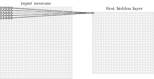
Each neuron in the first hidden layer will be connected to a small region of the input neurons, say, a $5 \times 5$ region, corresponding to 25 input pixels. That region in the input image is called the local receptive filed for the hidden neuron.

Then we slide the local receptive field over by one neuron to the right to connect to a second hidden neuron:

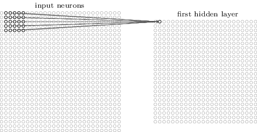
And so on, building the first hidden layer. Note that if we have $28 \times 28$ input image and $5 \times 5$ local receptive fields, then there will be $24 \times 24$ neurons in the hidden layer.

We've moved the local receptive field by 1 pixel at a time. Sometimes a different stride length is used.

These hyper-parameters such as the size of local receptive field and the stride length can be determined by the same approach as choosing other hyper-parameters: by benchmarking the best performance on the validation data.

Shared weights and biases

Each hidden neuron has a bias and $5 \times 5$ weights connected to its local receptive field. We are going to use the same weights and bias for each of the $24 \times 24$ hidden neurons. The output for the $j,k^\text{th}$ hidden neuron is:

$$ \begin{align} \sigma\left(b + \sum_{l=0}^4 \sum_{m=0}^4 w_{l,m} a_{j+l, k+m} \right), \tag{103} \end{align} $$

where $\sigma$ is the activation function, $b$ is the shared value for the bias, $w_{l,m}$ is a $5 \times 5$ array of shared weights, and we use $a_{x,y}$ to denote the input activation at position $x,y$.

This means that all the neurons in the first hidden layer detect exactly the same feature, just at different locations in the input image. The feature is the input pattern that will cause the neuron to activate: it might be an edge in the image, or some other shape. Convolutional networks are well adapted to the translation invariance of images.

For this reason we sometimes call the map from the input layer to the hidden layer a feature map. The shared weights and shared bias define the feature map. The feature map is sometimes called a kernel or filter.

We have just described a network that can detect a single kind of localized feature. To do image recognition, we'll need more than one feature map. A complete convolutional layer consists of several different feature maps:

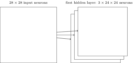
In the picture there are three feature maps. Each feature map is defined by a set of $5 \times 5$ shared weights and a single shared bias. The result is that the network can detect three different kinds of features, with each feature being detectable across the entire image. In practice convolutional networks may use more feature maps.

Gabor filter has been one of the traditional approaches to image recognition.

The big advantage of sharing weights and biases is that it greatly reduces the number of parameters learned in a convolutional network. If we have 20 feature maps, we have a total of $20 \times (5 \times 5 + 1) = 520$ parameters defining the convolutional layer. If we had a fully connected first layer of $28 \times 28 = 784$ input neurons and 30 hidden neurons, that would be a total of $784 \times 30 + 30 = 23,550$ parameters. That's more than 45 times as many parameters as the convolutional layer.

The use of translation invariance and reduced number of parameters results in faster training for the convolutional model.

Pooling layers

Pooling layers are usually used immediately after the convolutional layers. A pooling layer takes each feature map output from the convolutional layer and prepares a condensed feature map. For example, each unit in the pooling layer may summarize a region of $2 \times 2$ neurons in the previous layer. A common procedure for pooling is know as max-pooling, which outputs the maximum activation in the $2 \times 2$ input region:

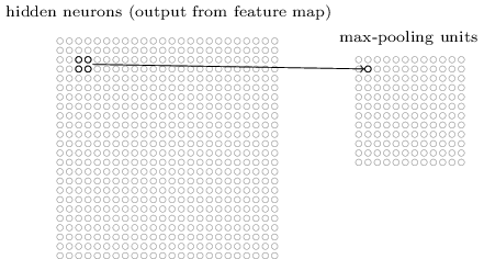
Note that if we have $24 \times 24$ neurons output from the convolutional layer, after pooling we have $12 \times 12$ neurons.

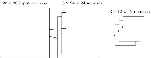
The convolutional layers usually have several feature maps. We apply max-pooling to each feature map separately:

We can think of max-pooling as a way for the network to determine whether a given feature is found anywhere in the region of the image. Once a feature has been found, its exact location isn't as important as its relative location to other features. This approach helps reduce the number of parameters needed in later layers.

Another common approach is known as L2 pooling, where we take the square root of the sum of the squares of the activations in the $2 \times 2$ region. This is another approach to condense information from the convolutional layer. We can test different pooling methods on the validation data to determine which one works best to optimize the performance.

Putting it all together

Now we can use the ideas of local receptive fields, shared weights and biases, and pooling layers to form a complete convolutional neural network. It is similar to the architecture that we have just discussed, but has an additional layer of 10 output neurons, corresponding to the 10 possible values for MNIST digits:

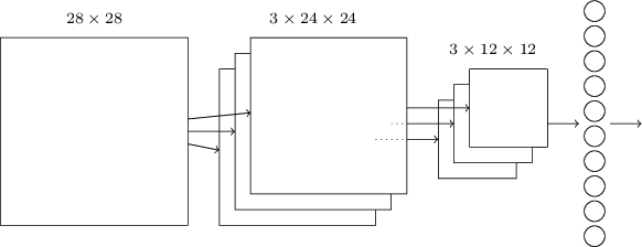
The network begins with $28 \times 28$ input neurons, which are used to encode the pixel intensities for the MNIST image. This is then followed by a convolutional layer using a $5 \times 5$ local receptive field and 3 feature maps. The result is a layer of $3 \times 24 \times 24$ hidden feature neurons. The next step is a max-pooling layer, applied to $2 \times 2$ regions, across each of the 3 feature maps. The result is a layer of $3 \times 12 \times 12$ hidden feature neurons.

The final layer is a fully connected layer: it connects every neuron from the max-pooled layer to every one of the 10 output neurons.

As earlier, we will use stochastic gradient descent and backpropagation to train our network. However, we need to modify the equation of backpropagation to accommodate the convolutional and max-pooling layers.

Implementing convolutional neural networks

We are going to use TensorFlow with Keras library to implement more complex deep networks because it will speed up the runtime.

model = keras.Sequential([
    layers.Dense(100, activation="sigmoid"),
    layers.Dense(10, activation="softmax")
])
model.compile(optimizer="SGD",
              loss="categorical_crossentropy",
              metrics=["accuracy"])
keras.optimizers.SGD(learning_rate=0.1)
model.fit(subtrain_images, subtrain_labels,
    epochs=60,
    batch_size=10,
    validation_data=(valid_images, valid_labels)
   )