Matrix-based implementation
Modern processors incorporate circuits that enable them to manipulate matrices in a single run. Instead of computing feedforward and backpropagation algorithms for each example in the dataset separately, we can speed up learning by computing the same operations for the whole mini-batch of data at once.
Loading MNIST data
In order to use the full power of matrix operations, we first need to add a helper function to the mnist program so that it returns matrices for training and testing datasets.
def load_matrix_data():
    """Returns preprocessed MNIST dataset in a matrix-based form. ``train_data``
    is a tuple (X_train, Y_train) representing the matrix of training inputs and
    the matrix of corresponding labels accordingly. ``test_data`` is a tuple
    (X_test, y_test) of the matrix of testing inputs and the vector of
    corresponding labels accordingly. Testing labels are not vectorized.
    X_train.shape=(60000, 784), Y_train.shape=(60000, 10)
    X_test.shape=(10000, 784), y_test.shape=(10000,)"""
    (train_images, train_labels) = load_train_data()
    (test_images, test_labels) = load_test_data()
    # preprocess train data
    train_images = train_images.reshape((60000, 28*28))
    train_images = train_images.astype('float64') / 255
    train_labels = vectorize(train_labels)
    train_labels = train_labels.reshape(-1,10)
    train_data = (train_images, train_labels)
    # preprocess test data (labels are not vectorized)
    test_images = test_images.reshape((10000, 28*28))
    test_images = test_images.astype('float64') / 255
    test_data = (test_images, test_labels)
    return (train_data, test_data)
Network class
For convenience, we will represent weights in a transposed form that will facilitate our later computations (such that every row of activation matrix corresponds to one example in the mini-batch). For example, \(W^3\) is a matrix such that \(w_{kj}^3\) is the weight for the connection between the \(k^{\text{th}}\) neuron in the second layer and the \(j^{\text{th}}\) neuron in the third layer.
Also, we will represent biases vector as a 1-dimensional numpy array so that it will be broadcaseted for every example in the mini-batch (original matrix representation doesn't allow broadcasting).
import numpy as np

class Network(object):
    def __init__(self, sizes, seed=None):
        """The list ``sizes`` contains the number of neurons in the
        respective layers of the network. For example, if the list
        was [3, 4, 2] then it would be a three-layer network, with the
        first layer containing 3 neurons, the second layer 4 neurons,
        and the third layer 2 neurons. The biases and weights for the
        network are initialized randomly, using a Gaussian
        distribution with mean 0 and variance 1. Note that the first
        layer is assumed to be an input layer, and by convention we
        won't set any biases for those neurons, since biases are only
        ever used in computing the outputs from later layers. Integer
        ``seed`` may be provided to achieve reproducible results."""
        self.rng = np.random.default_rng(seed)
        self.num_layers = len(sizes)
        self.biases = [self.rng.standard_normal(size=(j,), dtype=np.float64)
            for j in sizes[1:]]
        self.weights = [self.rng.standard_normal(size=(k, j), dtype=np.float64)
            for k, j in zip(sizes[1:], sizes[:-1])]
The advantage of this ordering is that we can multiply two matrices, weights \(W^l\) and activations \(A^{l-1}\) directly for the whole mini-batch (compare it to Equation (7)):
$$ \begin{align} A^{l} = \sigma(A^{l-1} W^l + b^l), \end{align} \tag{58} $$
where \(A^{l-1}\) is the matrix of activations such that \(a_{i,j}^{l-1}\) is the activation of the \(j\) neuron in the \((l-1)^\text{th}\) layer for example \(i\) in the mini-batch.
def feedforward(self, X):
    """Returns a matrix of activations in each layer in the network
    for the mini-batch. Each activation matrix j has the shape
    (mini_batch_size, sizes[j]), where sizes[j] is the number of neurons
    in the layer j. The biases vector is broadcasted to match
    the resultant matrix of multiplication of activations in the
    previous layer and weights in the current layer."""
    A = X
    # list to store all the activations, layer by layer
    Activations = [X]
    for b, W in zip(self.biases, self.weights):
        Z = np.matmul(A, W) + b # Equation (58)
        A = self.sigmoid(Z)
        Activations.append(A)
    return Activations
Stochastic gradient descent
After we get the training dataset in a matrix form and change weights and biases representation, we will modify the SGD function so that it can handle matrices. We will randomly permute two matrices of inputs and labels in unison for stochastic gradient descent which is accomplished by self.rng.shuffle function:
def SGD(self, train_data, epochs, mini_batch_size, eta,
        test_data=None):
    """Trains the neural network using mini-batch stochastic
    gradient descent. The ``train_data`` is a tuple of two
    matrices (X_train, Y_train) representing the training inputs and
    the corresponding labels. X_train.shape=(n_train_examples, n_features),
    Y_train.shape=(n__train_examples, n_labels). ``eta`` is the learning rate,
    ``test_data`` may be optionally provided to evaluate the learning
    process. It is defined in the same way as ``train_data`` except that
    the labels are not vectorized."""
    (X_train, Y_train) = train_data
    n = X_train.shape[0] # number of training examples
    mask = np.arange(n)
    for j in range(epochs):
        # shuffle training data randomly
        self.rng.shuffle(mask)
        X_train = X_train[mask]
        Y_train = Y_train[mask]
        # divide train data into mini-batches
        for m in range(0, n, mini_batch_size):
            self.update_mini_batch(X_train[m:m+mini_batch_size,:],
                Y_train[m:m+mini_batch_size,:], mini_batch_size, eta)
        # evaluate metrics
        if test_data:
            correct = self.evaluate(test_data)
            print(f"Epoch {j} : {correct} / {test_data[0].shape[0]}")
        else:
            print(f"Epoch {j} complete")
The update_mini_batch function has lost some of its code that is now handled by the backprop function:
def update_mini_batch(self, X_train, Y_train, mini_batch_size, eta):
    """Updates the network's weights and biases by applying
    gradient descent using backpropagation to a single mini-batch.
    The matrix ``X_train`` represents training inputs of the mini-batch,
    and the matrix ``Y_train`` represents its the desired outputs."""
    (nabla_b, nabla_w) = self.backprop(X_train, Y_train)
    self.biases = [b-(eta/mini_batch_size)*nb
                    for b, nb in zip(self.biases, nabla_b)] # Equation (25)
    self.weights = [w-(eta/mini_batch_size)*nw
                    for w, nw in zip(self.weights, nabla_w)] # Equation (24)
Backpropagation
The cost function for the mini-batch will be the sum of the cost of individual examples in the mini-batch. We can also represent it as a Frobenius norm of the difference matrix of labels and output activations for the mini-batch:
$$ \begin{align} C_m = \frac{1}{2} |Y_m-A^L|\text{F} = \frac{1}{2} \sum{i=1}^m \sum_{j=1}^k (y_{ij}-a_{ij}^L)^2, \tag{59} \end{align} $$
where \(C_m\) is the cost for the mini-batch, \(m\) is the number of examples in the mini-batch, \(k\) is the number of output neurons, \(Y_m\) is the matrix of labels for the mini-batch such that \(y_{ij}\) is the label \(j\) for example \(i\) in the mini-batch, \(A^L\) is the matrix of output activations such that \(a_{ij}^L\) is the activation for example \(i\) in the mini-batch from \(j\) output neuron.
Now we need to use matrix calculus to compute the derivative of the cost function with respect to the matrix of output activations:
$$ \begin{align} \nabla_{A^L} C_m = \frac{\partial C_m}{\partial A^L} = A^L-Y_m \tag{60} \end{align} $$
@staticmethod
def cost_derivative(output_Activations, Y_train):
    """Returns the matrix of partial derivatives dC_m/dA
    for the output activations."""
    return (output_Activations - Y_train) # Equation (60)
The weighted input \(Z^l\), analagous to the activation \(A^l\), will be represented in a matrix form, such that \(z_{ij}^l\) is the weighted input of neuron \(j\) in the \(l^\text{th}\) layer for example \(i\) in the mini-batch. The logistic sigmoid function is applied element-wize for every element in the matrix \(Z^l\) to obtain activation \(A^l\):
$$ \begin{align} A^l = \sigma(Z^l) \quad \text{s.t.} \quad a_{ij}^l = \frac{1}{1+e^{-z_{ij}^l}}. \tag{61} \end{align} $$
Since sigmoid is applied element-wise, computing its derivative is straightforward:
$$ \begin{align} \sigma'(z_{ij}^l) & = a_{ij}^l(1 - a_{ij}^l). \tag{62} \end{align} $$
Or, in matrix form:
$$ \begin{align} \sigma'(Z^l) & = A^l\odot(1 - A^l). \tag{63} \end{align} $$
In summary, the fundamental equations for backpropagation in matrix form are the following:
$$ \begin{align} \Delta^L = \frac{\partial C_m}{\partial Z^L} &= \nabla_{A^L} C_m \odot \sigma'(Z^L) \tag{MBP1}\\[2ex] \Delta^l = \frac{\partial C_m}{\partial Z^l} &= (\Delta^{l+1} (w^{l+1})^T) \odot \sigma'(Z^l) \tag{MBP2}\\[2ex] \frac{\partial C_m}{\partial b^l} &= (\mathbb{1}_m)^T \Delta^l \tag{MBP3}\\[2ex] \frac{\partial C_x}{\partial w^l} &= (A^{l-1})^T \Delta^l \, , \tag{MBP4} \end{align} $$
where \((\mathbb{1}_m)^T\) is a row vector of ones with number of elements \(m\), which by multiplying with \(\Delta^l\) effectively sums the error in layer \(l\) for all examples in the mini-batch. The backprop function now does most of the work of calculating gradients for weights and biases for each mini-batch:
def backprop(self, X_train, Y_train):
    """Returns a tuple ``(nabla_b, nabla_w)`` representing the
    gradient for the cost function C_m for the mini-batch. ``nabla_b``
    and ``nabla_w`` are layer-by-layer lists of numpy arrays,
    similar to ``self.biases`` and ``self.weights``."""
    nabla_b = [np.zeros(b.shape) for b in self.biases]
    nabla_w = [np.zeros(w.shape) for w in self.weights]
    Activations = self.feedforward(X_train) # matrix of activations
    # compute dC/dZ, dC/db, and dC/dw for the output layer
    dCdA = self.cost_derivative(Activations[-1], Y_train) # 1st term of MBP1
    spZ = self.sigmoid_prime(Activations[-1]) # 2nd term of MBP1
    Delta = np.multiply(dCdA, spZ) # MBP1
    nabla_b[-1] = np.sum(Delta, axis=0) # MBP3
    nabla_w[-1] = np.matmul(Activations[-2].transpose(), Delta) # MBP4
    # compute dC/dZ, dC/db, and dC/dw for all the previous layers
    for l in range(2, self.num_layers):
        Dw = np.matmul(Delta, self.weights[-l+1].transpose()) # 1st term of MBP2
        spZ = self.sigmoid_prime(Activations[-l]) # 2nd term of MBP2
        Delta =  np.multiply(Dw, spZ) # MBP2
        nabla_b[-l] = np.sum(Delta, axis=0) # MBP3
        nabla_w[-l] = np.matmul(Activations[-l-1].transpose(), Delta) # MBP4
    return (nabla_b, nabla_w)
The evaluate function now calculates the number of correctly identified examples using matrices instead of looking for every single entry in an array with a for loop.
def evaluate(self, test_data):
    """Returns the number of correctly identified examples."""
    (X_test, y_test) = test_data
    Activations = self.feedforward(X_test)
    correct = np.sum((np.argmax(Activations[-1], axis=1) == y_test).astype(int))
    return correct
Finally, we modified the sigmoid_prime function so that the element-wise multiplication for the matrix is done with the help of np.multiply routine:
def sigmoid_prime(self, A):
    """Returns the derivative of the sigmoid function."""
    return np.multiply(A, 1.0-A) # Equation (63)
The code is available at my GitHub repository.
Running the code
The effect of all these changes is a significant boost in speed of the computation. Depending on the complexity of the network, the improvement starts from a factor of six for 15 hidden neurons with mini-batch size of 10 to a factor of thirty for 100 hidden neurons network with a mini-batch size of 128.
Modern AI frameworks, such as Tensorflow and Pytorch, use Cuda programming to optimize matrix manipulations of artificial neural networks for parallel GPU computation. GPUs have more processing units than CPUs by a factor of 1,000 so that the speed of computation is increased even further.
import mnist
(train_data, test_data) = mnist.load_matrix_data()
net = Network([784, 15, 10], seed=0)
net.SGD(train_data, 30, 10, 3.0, test_data)
Comparing to other implementations
We mentioned that our program performs well, but it is good to actually compare it to other possible implementations. The simplest baseline program is to guess the digit randomly. The accuracy will be about 10 percent.
But we can do better than that: we can look at how dark an image is. For example, an image of a 2 will be typically darker than an image of 1. So we can compute the average darkness for each digit and compare it to the new image to determine which image has the closest average darkness. This way we get about 22.25 percent accuracy.
We can think of many other ideas and get up over 50 percent accuracy. But to get much higher accuracy we have to use established machine learning algorithms, such as the support vector machine or SVM for short.
We will use Python library called scikit-learn which provides a simple Python interface to a fast C-based library for SVM known as LIBSVM. If we run scikit-learn SVM classifier using the default settings, then it gets 9,785 of 10,000 test images correct. It is possible to improve SVM by tuning its parameters.
However, well-designed neural networks outperform every other technique for solving MNIST, including SVMs. The current record is classifying 9,979 of 10,000 images correctly. This was done by Li Wan, Matthew Zeiler, Yann LeCun, and Rob Fergus.
Toward deep learning
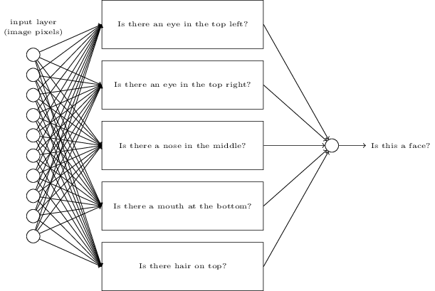
Suppose we want to build a network which answers a very complicated question: is a given image a face or not. Forgetting about neural networks for a moment, we might want to break the problem into sub-problems: does the image have an eye in the top left? Does it have an eye in the top right? Does it have a nose in the middle? And so on.
If the answers to several of these questions are "yes", or even just "probably yes", then we can conclude that the image is likely to be a face. Conversely, if the answers to most of the questions are "no", then the image probably is not a face.
Heuristic suggests that if we can solve sub-problems by using neural networks, then perhaps we can build a neural network for face detection by combining the networks for the sub-problems.
Here is a possible architecture with rectangle denoting the sub-problems:
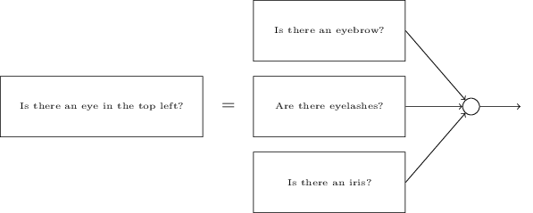
It is also plausible that sub-networks can be decomposed. Suppose we are considering the question: "Is there an eye in the top left?" This can be decomposed into questions such as: "Is there an eyebrow?"; "Are there eyelashes?"; "Is there an iris?"; and so on. These questions should also include positional questions but let's keep it simple. The network to ask the question "Is there an eye in the top left?" can now be decomposed:
Those questions too can also be broken down further and further through multiple layers. In the end, we will be working with sub-networks that answer questions so simple they can easily be answered at the level of single pixels. These questions might, for example, be about the presence or absence of very simple shapes at particular points in the image. Such questions can be answered by single neurons connected to the raw pixels in the image.
Networks with this kind of many-layer structure - two or more hidden layers - are called deep neural networks. Deep neural networks with 5 to 10 hidden layers perform much better than shallow neural networks that have only a single hidden layer. The reason is the ability of deep neural nets to build up a complex hierarchy of concepts. The learning techniques for deep learning are based on stochastic gradient descent and backpropagation. Contrary to the research in 1980s and 1990s, contemporary approach uses new ideas to improve learning performance.
Adapted from Michael A. Nielsen, "Neural Networks and Deep Learning"