Backpropagation

Hadamard product

Suppose vectors $s$ and $t$ are of the same dimension. We will use $s \odot t$ to denote the elementwise product of the two vectors, which is also known as the Hadamard product. For example:

$$ \begin{align} \left[\begin{array}{c} 1 \\ 2 \end{array}\right] \odot \left[\begin{array}{c} 3 \\ 4 \end{array} \right] = \left[ \begin{array}{c} 1 \cdot 3 \\ 2 \cdot 4 \end{array} \right] = \left[ \begin{array}{c} 3 \\ 8 \end{array} \right]. \tag{34} \end{align} $$

The error measure

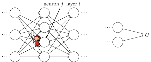
Backpropagation is about understanding how changing the weights and biases in a network changes the cost function. Ultimately this means computing partial derivatives $\partial C_x / \partial w_{jk}^l$ and $\partial C_x / \partial b_j^l$. But to compute those, we first introduce an intermediate quantity $\delta^l_j$, which we call the error in the $j^{\text{th}}$ neuron in the $l^{\text{th}}$ layer (we can also describe it as the change in $C_x$ with respect to the change in the weighted input to the neuron $z_j^l$). Backpropagation will give us a procedure to compute the error $\delta^l_j$, and then we will relate $\delta^l_j$ to $\partial C_x / \partial w_{jk}^l$ and $\partial C_x / \partial b_j^l$.

Suppose we want to change $z_j^l$ at the $j^{\text{th}}$ neuron in layer $l$ by $\Delta z^l_j$. Instead of outputting $\sigma(z^l_j)$, the neuron now outputs $\sigma(z^l_j+\Delta z^l_j)$. This change propagates through later layers in the network, finally causing the overall cost to change by an amount $ \Delta C_x \approx \frac{\partial C_x}{\partial z^l_j} \Delta z^l_j$, which is given by the linear approximation. When we take the limit when $\Delta z^l_j$ approaches zero, the relationship becomes exact instead of being approximate. If we choose $\Delta z^l_j$ such that its sign is opposite to $\frac{\partial C_x}{\partial z^l_j}$, then we can lower the cost quite a bit. However, if $\frac{\partial C_x}{\partial z^l_j}$ is close to zero, then we cannot improve the cost much by perturbing the weighted input $z_j^l$.

Now we define the error $\delta_j^l$ of neuron $j$ in layer $l$ by

$$ \begin{align} \delta_j^l \equiv \frac{\partial C_x}{\partial z_j^l}. \tag{35} \end{align} $$

We will use $\delta^l$ to denote the vector of errors associated with layer $l$. Backpropagation will give us a way of computing $\delta^l$ for every layer, and then we will relate those errors to the quantities of real interest, $\partial C_x / \partial w_{jk}^l$ and $\partial C_x / \partial b_j^l$. Backpropagation is based on four fundamental equations.

An equation for the error in the output layer

Using the chain rule of calculus we can easily compute the error in the output layer $\delta^L$ as following:

$$ \begin{align} \delta_j^L = \sum_k \frac{\partial C_x}{\partial a_k^L} \frac{\partial a_k^L}{\partial z_j^L}, \tag{36} \end{align} $$

where the sum is over all neurons $k$ in the output layer. However, the output activation $a_k^L$ of the $k^{\text{th}}$ neuron depends on the weighted input $z_j^L$ for the $j^{\text{th}}$ neuron only when $k = j$. Therefore, the derivative $\frac{\partial a_k^L}{\partial z_j^L}$ equals zero when $k \ne j$. As a result, we can simplify the previous equation to

$$ \begin{align} \delta_j^L = \frac{\partial C_x}{\partial a_j^L} \frac{\partial a_j^L}{\partial z_j^L}. \tag{37} \end{align} $$

Recall that $a_j^L = \sigma(z_j^L)$, therefore we can rewrite the equation (37) as:

$$ \begin{align} \delta_j^L = \frac{\partial C_x}{\partial a_j^L} \sigma'(z_j^L). \tag{38} \end{align} $$

The first term on the right, $\frac{\partial C_x}{\partial a_j^L}$, measures how fast the cost is changing as a function of the $j^{\text{th}}$ output activation. For example, if $C_x$ does not depend much on a particular output neuron $j$, then $ \delta_j^L$ will be small. The second term on the right, $\sigma'(z^L_j)$, measures how fast the activation function $\sigma$ is changing at the weighted input to the neuron $z_j^L$.

Notice that everything in Equation (38) is easily computed. We compute $z_j^L$ while performing feedforward calculations. Computing the derivative of the quadratic cost function is very easy. Recall from Equation (10) that

$$ \begin{align} C_x = \frac{1}{2} \sum_j (y_j-a_j^L)^2. \end{align} $$

Now we will calculate the derivative of the quadratic cost function:

$$ \begin{align} \nabla_a C_x = \frac{\partial C_x}{\partial a_j^L} = a_j^L - y_j \tag{39} \end{align} $$

Computing $\sigma'(z^L_j)$ is also easy. Recall from equation (3) that

$$ \begin{align} \sigma(z_j^L) \equiv \frac{1}{1+e^{-z_j^L}}. \end{align} $$

Now we can calculate the derivative of the sigmoid function:

$$ \begin{align} \sigma'(z_j^L) & = \frac{-1}{(1+e^{-z_j^L})^2} \cdot e^{-z_j^L} \cdot (-1)\\ & = \frac{e^{-z_j^L}}{(1+e^{-z_j^L})^2}\\ & = \frac{1}{1+e^{-z_j^L}} \cdot \left( 1 - \frac{1}{1+e^{-z_j^L}} \right)\\[2ex] & = \sigma(z_j^L) (1 - \sigma(z_j^L))\\[2ex] & = a_j^L(1 - a_j^L). \tag{40} \end{align} $$

Equation (38) is a componentwise expression for $\delta^L$ which we can rewrite in a matrix-based form using previously described Hadamard product:

$$ \begin{align} \delta^L = \nabla_a C_x \odot \sigma'(z^L). \tag{BP1} \end{align} $$

Here, $\nabla_a C_x$ is the gradient vector of the cost function with respect to the output vector $a$. It is the rate of change of $C_x$ with respect to the output activations, and its components are $\frac{\partial C_x}{\partial a_j^L}$. In the case of quadratic cost function we have $\nabla_a C_x = (a^L - y)$, therefore the fully matrix-based form is:

$$ \begin{align} \delta^L & = (a^L - y) \odot \sigma'(z^L)\\[2ex] & = (a^L - y) \odot (a^L \odot (1 - a^L)). \tag{41} \end{align} $$

Notice that we can easily add a scalar to a vector with existing rules of linear algebra.

An equation for the error in a previous layer

Next we will derive an equation for the error $\delta^l$ in terms of the error in the next layer $\delta^{l+1}$ by using the chain rule of calculus:

$$ \begin{align} \delta_j^l & = \frac{\partial C_x}{\partial z_j^l}\\ & = \sum_k \frac{\partial C_x}{\partial z_k^{l+1}} \frac{\partial z_k^{l+1}}{\partial z_j^l}\\ & = \sum_k \delta_k^{l+1} \frac{\partial z_k^{l+1}}{\partial z_j^l}, \tag{42} \end{align} $$

where the sum is over all neurons $k$ in the $(l+1)^{\text{th}}$ layer. We have to sum all the neurons in the $(l+1)^{\text{th}}$ layer because the output from each neuron in the current $l^{\text{th}}$ layer is fed into all the neurons in the $(l+1)^{\text{th}}$ layer. Notice that we have substituted the definition of $\delta_k^{l+1}$ on the right side of Equation (42).

Next we will evaluate the second term from the expression for $z_k^{l+1}$ (consider $k$ as one of the neurons in the $(l+1)^{\text{th}}$ layer):

$$ \begin{align} z_k^{l+1} = \sum_j w_{kj}^{l+1} a_j^l +b_k^{l+1} = \sum_j w_{kj}^{l+1} \sigma(z_j^l) +b_k^{l+1}, \tag{43} \end{align} $$

where the sum is over all neurons $j$ in the current $l^{\text{th}}$ layer. Notice that $w_{kj}^{l+1}$ is a weight on connection from the $j$ neuron in the $l^{\text{th}}$ layer to the $k$ neuron in the $(l+1)^{\text{th}}$ layer. After taking the derivative on both sides with respect to $z_j^l$, we obtain

$$ \begin{align} \frac{\partial z_k^{l+1}}{\partial z_j^l} = w_{kj}^{l+1} \sigma'(z_j^l). \tag{44} \end{align} $$

Notice that when we take the derivative of $z_k^{l+1}$ with respect to $z_j^l$, only one particular $z_j^l$ survives in the derivation process, so we can get rid of the sum over all other $j$'s. Put it another way, when we consider how the output from one neuron in the $l^{\text{th}}$ layer affects the weighted input of one particular neuron in the $(l+1)^{\text{th}}$ layer, only this one neuron in the $l^{\text{th}}$ layer under consideration matters. Substituting back into the Equation (42), we obtain

$$ \begin{align} \delta_j^l = \sum_k \delta_k^{l+1} w_{kj}^{l+1} \sigma'(z_j^l), \tag{45} \end{align} $$

where the sum is over all neurons $k$ in the $(l+1)^{\text{th}}$ layer.

We can represent the Equation (45) in the matrix-based form as the following:

$$ \begin{align} \delta^l = ((w^{l+1})^T \delta^{l+1}) \odot \sigma'(z^l), \tag{BP2} \end{align} $$

where $(w^{l+1})^T$ is the transpose of the weight matrix $w^{l+1}$ for the $(l+1)^{\text{th}}$ layer.

By combining (BP1) and (BP2) we can compute the error $\delta^l$ for any layer in the network. We start with (BP1) to compute $\delta^L$, then apply equation (BP2) to compute $\delta^{L-1}$, then apply equation (BP2) again to compute $\delta^{L-2}$, and so on all the way back through the network.

An equation for the rate of change of the cost with respect to the bias

Recall from equation (8) that the vectorized weighted input to the neurons in layer $l$ is

$$ \begin{align} z^l \equiv w^l a^{l-1}+b^l. \end{align} $$

We can modify this equation to show the components of the weighted input $z_j^l$ to make it more clear:

$$ \begin{align} z_j^l = \sum_k w_{jk}^l a_k^{l-1} + b_j^l, \end{align} \tag{46} $$

where the sum is over all neurons $k$ in the $(l-1)^{\text{th}}$ layer. We notice that the coefficient of the bias $b_j^l$ is 1, which means that:

$$ \begin{align} \frac{\partial z_j^l}{\partial b_j^l} = 1 \end{align} \tag{47} $$

Applying the chain rule, we can determine the rate of change of the cost function with respect to any bias in the network as following:

$$ \begin{align} \frac{\partial C_x}{\partial b_j^l} = \frac{\partial C_x}{\partial z_j^l} \frac{\partial z_j^l}{\partial b_j^l} = \delta_j^l \cdot 1 = \delta_j^l. \tag{48} \end{align} $$

In vectorized form, Equation (48) will become the following simple expression:

$$ \begin{align} \frac{\partial C_x}{\partial b^l} = \delta^l. \tag{BP3} \end{align} $$

An equation for the rate of change of the cost with respect to the weight

We will use the Equation (46) to determine the relationship of a particular weight $w_{jk}^l$ to the weighted input $z_j^l$:

$$ \begin{align} z_j^l = \sum_k w_{jk}^l a_k^{l-1} + b_j^l, \end{align} $$

where the sum is over all neurons $k$ in the $(l-1)^{\text{th}}$ layer. If we take the derivative of $z_j^l$ with respect to a particular weight $w_{jk}^l$ in the same layer, we notice that all other weights in the sum will vanish together with the bias $b_j^l$:

$$ \begin{align} \frac{\partial z_j^l}{\partial w_{jk}^l} = a_k^{l-1}. \tag{49} \end{align} $$

Applying the chain rule, we can calculate the rate of change of the cost function with respect to the weight as follows:

$$ \begin{align} \frac{\partial C_x}{\partial w_{jk}^l} = \frac{\partial C_x}{\partial z_j^l} \frac{\partial z_j^l}{\partial w_{jk}^l} = \delta_j^l a_k^{l-1}. \tag{50} \end{align} $$

Notice that $a_k^{l-1}$ is a scalar when we differentiate a particular weighted input $z_j^l$ to a particular weight $w_{jk}^l$ so the order does not matter. However, in the vectorized form we need to take a transpose of $a^{l-1}$ to obtain a matrix that will match the shape of the weights matrix:

$$ \begin{align} \frac{\partial C_x}{\partial w^l} = \delta^l (a^{l-1})^T. \tag{BP4} \end{align} $$

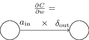
To get a better picture of what is happening with the rate of change of the cost with respect to a particular weight, we can rewrite Equation (50) in a less index-heavy notation as

$$ \begin{align} \frac{\partial C_x}{\partial w} = a_{\text{in}} \delta_{\text{out}}, \tag{51} \end{align} $$

where $a_{\text{in}}$ is the activation of the neuron input to the weight $w$, and $\delta_{\text{out}}$ is the error of the neuron output from the weight $w$. Zooming in to look at a particular weight $w$ and two neurons connected by that weight, we can depict this as:

A consequence of this equation is that when the activation $a_{\text{in}}$ is small, $a_{\text{in}} \approx 0$, the gradient term $\frac{\partial C_x}{\partial w}$ will also tend to be small. In this case, we say that the weight learns slowly, meaning it is not changing much during gradient descent.

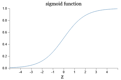
Also, recall the graph of the sigmoid function $\sigma$. It becomes very flat when $\sigma(z_j^L)$ is approximately 0 or 1. When this occurs, its derivative $\sigma'(z_j^L) \approx 0$. Therefore, a weight and bias in the final layer will learn slowly if the output neuron is either low activation ($\approx 0$) or high activation ($\approx 1$). In this case we say that the output neuron has saturated, and as a result, the weight and bias have stopped learning (or learning slowly). The similar conclusions may be made for earlier layers, unless $({w^{l+1}})^T \delta^{l+1}$ (recall Equation (BP2)) is large enough to compensate for the small values of $\sigma'(z_j^l)$.

Summary of the equations

To sum up, we have learnt that a weight will learn slowly if either the input neuron is low-activation, or if the output neuron has saturated, i.e. is either high- or low-activation.

It is worth to mention that the four fundamental equations hold for any cost and activation functions, not just the sigmoid and quadratic cost functions, so we can use these equations to design cost and activation functions which have desired learning properties which prevents saturation of sigmoid neurons.

$$ \begin{align} \delta^L = \frac{\partial C_x}{\partial z^L} &= \nabla_a C_x \odot \sigma'(z^L) \tag{BP1}\\[2ex] \delta^l = \frac{\partial C_x}{\partial z^l} &= ((w^{l+1})^T \delta^{l+1}) \odot \sigma'(z^l) \tag{BP2}\\[2ex] \frac{\partial C_x}{\partial b^l} &= \delta^l \tag{BP3}\\[2ex] \frac{\partial C_x}{\partial w^l} &= \delta^l (a^{l-1})^T. \tag{BP4} \end{align} $$

Backpropagation algorithm

The backpropagation equations provide us with a way of computing the gradient of the cost function. Now we will express this in the form of an algorithm:

1. Input $x$: Set the activation function $a^1$ for the input layer.

2. Feedforward: For each layer $l = 2, 3, \ldots, L$ compute $z^l = w^l a^{l-1}+b^l$ and $a^{l} = \sigma(z^l)$.

3. Output error $\delta^L$: Compute the vector $\delta^L = \nabla_a C_x \odot \sigma'(z^L)$.

4. Backpropagate the error: For each $l = L-1, L-2, \ldots, 2$ compute $\delta^l = ((w^{l+1})^T \delta^{l+1}) \odot \sigma'(z^l)$.

5. Output: The gradient of the cost function is given by $\frac{\partial C_x}{\partial w^l} = \delta^l (a^{l-1})^T$ and $\frac{\partial C_x}{\partial b^l} = \delta^l$.

The algorithm is called backpropagation because we compute the errors $\delta^l$ backward, starting from the final layer. The backward movement is the consequence of the fact that cost is a function of outputs from the network, and to obtain earlier weights and biases we need to repeatedly apply the chain rule, working backward through the layers.

The backpropagation algorithm computes the gradient of the cost function for a single training example, $C_x$. In practice we need to combine backpropagation with a learning algorithm such as stochastic gradient descent, in which we compute the gradient for many training examples. In particular, given a mini-batch of $m$ training examples, the following algorithm applies a gradient descent learning step based on that mini-batch:

1. Input a set of training examples

2. For each training example $x$: Set the corresponding input activation $a^{x,1}$, and perform the following steps:

   • Feedforward: For each layer $l = 2, 3, \ldots, L$ compute $z^l = w^l a^{l-1}+b^l$ and $a^{l} = \sigma(z^l)$.

   • Output error $\delta^L$: Compute the vector $\delta^L = \nabla_a C_x \odot \sigma'(z^L)$.

   • Backpropagate the error: For each $l = L-1, L-2, \ldots, 2$ compute $\delta^l = ((w^{l+1})^T \delta^{l+1}) \odot \sigma'(z^l)$.

3. Gradient descent: For each $l = L-1, L-2, \ldots, 2$ update the weights according to the rule $w^l \rightarrow w^l - \frac{\eta}{m} \sum_x \delta^{x,l} (a^{x,l-1})^T$ and the biases according to the rule $b^l \rightarrow b^l - \frac{\eta}{m} \sum_x \delta^{x,l}$.

To implement stochastic gradient descent in practice we also need an outer loop that generates mini-batches of training examples, and another outer loop stepping through multiple epochs of training.

Remarks on the chain rule

The derivative of the cost function with respect to the weights in the output layer:

$$ \begin{align} \frac{\partial C_x}{\partial w_{jk}^L} = \frac{\partial C_x}{\partial a_j^L} \frac{\partial a_j^L}{\partial z_j^L} \frac{\partial z_j^L}{\partial w_{jk}^L} \, , \tag{52} \end{align} $$

where $w_{jk}^L$ is the weight from the neuron $k$ in the $(L-1)^\text{th}$ layer to the neuron $j$ in the $L^\text{th}$ layer. The derivative of the cost function with respect to the weights in the previous layer:

$$ \begin{align} \frac{\partial C_x}{\partial w_{kp}^{l-1}} = \frac{\partial C_x}{\partial a_j^l} \frac{\partial a_j^l}{\partial a_k^{l-1}} \frac{\partial a_k^{l-1}}{\partial z_k^{l-1}} \frac{\partial z_k^{l-1}}{\partial w_{kp}^{l-1}} \, , \tag{53} \end{align} $$

where $w_{kp}^{l-1}$ is the weight from the neuron $p$ in the $(l-2)^\text{th}$ layer to the neuron $k$ in the $(l-1)^\text{th}$ layer. We can expand the term $\frac{\partial a_j^l}{\partial a_k^{l-1}}$ as the following. Recall that $a_j^l= \sigma(z_j^l)$ and $z_j^l = \sum_k w_{jk}^l a_k^{l-1} + b_j^l$. Then

$$ \begin{align} \frac{\partial a_j^l}{\partial z_j^l} = \sigma'(z_j) \tag{54} \end{align} $$

$$ \begin{align} \frac{\partial z_j^l}{\partial a_k^{l-1}} = w_{jk}^l \tag{55} \end{align} $$

Then

$$ \begin{align} \frac{\partial a_j^l}{\partial a_k^{l-1}} & = \frac{\partial a_j^l}{\partial z_j^l} \frac{\partial z_j^l}{\partial a_k^{l-1}}\\[2ex] & = \sigma'(z_j) w_{jk}^l \tag{56} \end{align} $$

Now we can generalize to any layer:

$$ \begin{align} \frac{\partial C_x}{\partial w_{qr}^{i}} = \frac{\partial C_x}{\partial a_j^L} \underbrace{ \frac{\partial a_j^L}{\partial a_k^{L-1}} \frac{\partial a_k^{L-1}}{\partial a_p^{L-2}} \ldots \frac{\partial a_q^{i+1}}{\partial a_r^i} }_\text{from layer $L$ to layer $i$} \frac{\partial a_r^i}{\partial z_r^i} \frac{\partial z_r^i}{\partial w_{qr}^i} \, , \tag{57} \end{align} $$

where $w_{qr}^{i}$ is the weight from the neuron $r$ in the $i^\text{th}$ layer to the neuron $q$ in the $(i+1)^\text{th}$ layer.

Adapted from Michael A. Nielsen, "Neural Networks and Deep Learning"